Download
1 / 11
110 likes | 222 Views
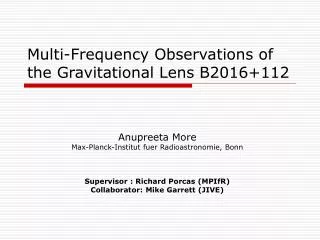
Multi-Frequency Observations of the Gravitational Lens B2016+112. Anupreeta More Max-Planck-Institut fuer Radioastronomie, Bonn Supervisor : Richard Porcas (MPIfR) Collaborator: Mike Garrett (JIVE). Outline. Introduction Background Koopmans scenario VLBI Observations 18cm, 6cm and 3.6cm

E N D
Multi-Frequency Observations of the Gravitational Lens B2016+112 Anupreeta More Max-Planck-Institut fuer Radioastronomie, Bonn Supervisor : Richard Porcas (MPIfR) Collaborator: Mike Garrett (JIVE)
Outline • Introduction • Background • Koopmans scenario • VLBI Observations • 18cm, 6cm and 3.6cm • Results • Summary
A ~ 3.4 arcsec B D (z=1.01) Source z = 3.27 C B2016+112 Courtsey: CASTLES website MERLIN map at 6cm
Koopmans Scenario • C is a pair of images of a part of the background source • C has a high magnification ~ 300 double quad Host galaxy of background source caustic D Radio Optical Koopmans et al. (2002)
My Work Spectral Analysis of Image A , Image B and Region C with the help of -- GLOBAL VLBI observations at 18cm and 6cm HSA observations at 3.6cm • To look for any counterparts of Region C components in Images A and B which will confirm Koopmans Scenario
a5 10 mas 10 mas a2 a4 a1 a3 b5 b2 b3 b4 b1 18cm 6cm 3.6 cm A B
C2-2 C2-1 C1-1 C1-2 50 mas C 18 cm 6 cm 3.6 cm
Frequency (GHz) Spectra of components in Image A
Summary • High resolution maps reveal more subcomponents in Images A and B demonstrating the expected opposite parity • Similarity in the spectra of C with the north-west sub-components in A and B are consistent with the Koopmans scenario