Download
1 / 28
290 likes | 459 Views
Interstellar turbulent plasma spectrum from multi-frequency pulsar observations. Smirnova T. V. Pushchino Radio Astronomy Observatory Astro Space Center P.N. Lebedev Physical Institute. 1. Relations of pulsar observations to the turbulent plasma spectrum

E N D
Interstellar turbulent plasma spectrum from multi-frequency pulsar observations Smirnova T. V.Pushchino Radio Astronomy ObservatoryAstro Space CenterP.N. Lebedev Physical Institute
1. Relations of pulsar observations to the turbulent plasma spectrum 2. Construction of the structure function • from multi-frequency observations 3. Measurements of the ISM spectrum in the directions to PSR 0329+54, 0437-47, 0809+74, 0950+08, 1642-03 • 4. Conclusions
Diffractive scintillation Inhomogeneities of size sd = /2sc ~ 107 1010 cm Time scale td = sd/V ~ sec min Frequency scale fd = c/(Rsc2) ~ KHz MHz Modulation index, m 1 Refractive scintillation Inhomogeneities of size sr = Rsc ~ 1012 1015 cm Time scale Tref = sr/V ~ weeks months srsd ~ R (Frenel scale)2 Dispersive arrival times, angular broading, time of arrival fluctuations, pulse broading
Electron density irregularities in the plasma cause random phase perturbations of the wavefront. These are characterized by the phase structure function: Ds() = <[S(1 +) – S(1)]2> S = const(f0/f)DM For a power-law spectrum Ne (q) = CNe2q-n, 2/li q 2/lout n = 11/3 for Kolmogorov spectrum Ds() =const2CNe2()n-2, q = 1/ Diffractive scintillation Correlation function of flux variations I(t) is described by the equation BI(t) = <I>2exp[- DS(t)] . If t0 is the characteristic scale of intensity variations we have DS(t0) = 1 DS(t) [BI(0) – BI(t)]/<I>2 (1/2) DI(t)/<I>2, t << t0 DS(t) DS() by = Vt
In frequency domain: DS(f) (n-2) [BI(0) – BI(f)]/<I>2 To reduce DS(f) to frequency f0 : DS(f , f0) = (f/f0)2DS(f,f) f(f0) = (f0/f)2f(f) For the case of strong angular refraction, ref >> dif: f(f0) = (f0/f)3f(f), ref = 3Vf/R(t/f) The slope of DS(f ) is the same as DS(t)
Refractive scintillation For homogeneous medium Ds() = mref2/(6(4-n))(Tref/tdif)2 = VTref Variations of DM DDM() = A (f0 / f)2<[DM(1+ ) – DM(1)]2>, A = 6,38.1014pc-2cm6 Pulsar timing Ds(t) = (2f)2 2τ2
dash line: n = 3.5 straight line: n = 11/3
Interstellar plasma spectrum in the direction to PSR 0329+54, Shishov, Smirnova, Siber et al., 2003R = 1 kpc, V = 95 km/s (parallax) Data: f = 102, 610, 4860 MHzFlux variations, Tref =17 days, m=0.37 at 610 MHz (Stinebring et al., 2000) Timing during 30 years, residuals t = 0.7 ms at 103 MHz (Shabanova, 1995) Reference frequency f0 = 1000 MHz
= 1.47 = 1.47 = 1.47 = 1.47
straight line: 1.5 dash line: 1.67
Interstellar plasma spectrum in the direction to PSR 1642-03, Smirnova, Shishov, Siber et al., A&A, 2006. Data: f = 102, 340, 610, 800, 4860 MHz = 30 mas/year (Brisken et al., 2003), R – 160 pc ? R = 160 pc, V = 22 km/s; R = 2.9 kpc, V = 400 km/s sc = 6.8 mas at 326 MHz (Gwinn et al., 1993) Flux variations, Tref = 0.9 days, m = 0.46 at 610 MHz (Stinebring et al., 2000) Timing during 8.5 years, residuals t = 1 ms at 103 MHz (Shabanova et al, 2001)
Interstellar plasma spectrum in the direction to PSR 0437-47 (Smirnova, Gwinn, Shishov, A&A, 2006R = 150 pc, V = 100 km/s (parallax) Data: f = 152, 327, 436 MHz fdif = 16 MHz, tdif = 17 min at 328 MHz (Gwinn et al. 2006)
PSR 0809+74R = 433 pc, V = 102 km/s (Brisken et al. 2002)Observations: f = 41, 62.43, 88.57 and 112.67 MHzDecember - January 2001, 2003, 2004 DKR: time duration 35.3 min BSA: T = 12 minTime resolution 2.56 ms or 5.12 msB = 12820 KHz and 128 1.25 KHz at 41 MHzTime averaging 19.4 s (15 P1) at 113 MHz, 39 s at 88 MHz,62 and 41 MHz
PSR 0950+08R = 262 pc, V = 36.6 km/s (Brisken et al. 2002)Observations: f = 41, 62.43, 88.57 and 112.67 MHzDecember - January 2001, 2003, 2004 DKR: time duration 15.63 min BSA: T = 3.2 minTime resolution 2.56 ms or 5.12 msB = 12820 KHz and 128 1.25 KHz at 41 MHzTime averaging 15.2 s (60 P1) at 113 MHz, 20.24 s at 88 MHz,62 and 41 MHz
Conclusions • Multi-frequency observations of pulsar interstellar scintillation give us new and more accurate information about the shape of turbulent spectrum in the definite directions of the sky. • 2. Interstellar plasma spectrum for 4 from 5 pulsars is well described by a power law with n from 3 to 3.5 for scales from 107 to 1010 cm which is different from Kolmogorov one. • 3. We detected strong angular refraction of radiation in the direction to 3 pulsars: 0329+54, 0437-47 and 0950+08. • 4. The spectrum in the direction to PSR 1642-03 has a changing of slope from n = 3.3 for scales less than 109 cm to n = 3.7 for scales from 109 to 1015 cm (Kolmogorov spectrum).