Download
1 / 35
350 likes | 461 Views
Boundary Point Elimination: A Path to Structure Aware SAT-solvers. Eugene Goldberg Northeastern University, USA. Algorithms and Applications for Next Generation SAT-solvers Dagstuhl, Germany 2009. Funded in part by SRC. Outline. Introduction Boundary Points and Resolution

E N D
Boundary Point Elimination: A Path to Structure Aware SAT-solvers Eugene Goldberg Northeastern University, USA Algorithms and Applications for Next Generation SAT-solvers Dagstuhl, Germany 2009 Funded in part by SRC
Outline • Introduction • Boundary Points and Resolution • IBP-SAT (SAT-solving with Interpolation by Boundary Point elimination) • Experimental Results • IBP-SAT and SAT-solvers with conflict clause learning • Conclusions
A Flaw of Modern SAT-Solvers Considerable progress has been achieved in using some types of structural information (e.g. certain types of symmetry) by SAT-solvers. However, they are still not very receptive to many kinds of structural information (like high-level structure of the formula). Modern SAT-solvers can achieve a much greater degree of scalability by making full use of the available structural information.
Can a SAT-solver Be Scalable? • Most likely NP ≠ P. Can a SAT-solver be scalable? • NP ≠ P just means that there can not exist an effi-cient black box SAT-solver. • Providing SAT-solvers with additional information(e.g. high-level structure and symmetry ) can make them scalable.
A Flaw of Conflict Driven Resolution Aflaw of the DPLL procedure and its derivatives: An individual resolution operation enters a proof only in a “package” (a set of resolutions describing a conflict). A resolution proof of a DPLL-like procedure already has a conflict induced structure ( ≠ formula’s structure).
A Simple Example Let C1= w v and C2 = ~w s be clauses of F. d=1 v=0 s=1 C2 C1 v=0 s=0 w=1 C1 C2 No conflict on variable w w=1 w=0 Conflict on variable w. Assignment v=0 and/or s=0 is implied A conflict set of clauses cannot consist only of C1 and C2
Resolution and Boundary Points In a DPLL-based procedure a single resolution is “meaningless”. It makes sense only as a part of a conflict clause derivation process. A potential solution to this problem: view a resolution proof as a procedure for elimination of boundary points (Goldberg , SAT-2009). Then even a single resolution operation removing a boundary point makes sense.
SAT-Solving with Interpolation By Boundary Point Elimination (IBP-SAT) • IBP-SAT builds a proof by elimination of boundary points by resolution operations. So this proof consists of “individual” resolutions. • IBP-SAT does use a DPLL-based procedure for finding boundary points. But the conflict clauses learned by it are not a part of the proof. • We show experimentally that IBP-SAT conside-rably outperforms DPLL-based SAT-solvers on the class of narrow formulas. Their structure is specified by variable ordering.
Conflict Clause Generation is a Special Case of IBP procedure Conf. driv. SAT-solver: F F1,..,Fk where Fi is a set of clauses responsible for a conflict. Resolving out variables of Fi in an order conflict clause Ci. IBP-SAT: F F1,..,Fk . Eliminating boundary points from Fi a set of clauses (generated by IBP-procedure). • The conflict clause generation procedure is a special case of the IBP-procedure used by IBP-SAT. • A set of clauses responsible for a conflict is not a narrow formula!!!
The Points We Are Making • We give an example of a successful SAT-algorithm that is not conflict driven!!!! • Taking into account structural information is crucial for building scalable SAT-algorithms. • Boundary point elimination seems to be a viable approach to building resolution proofs. • IBP-SAT is a generalization of SAT-solvers with conflict driven learning.
Outline • Introduction • Boundary Points and Resolution • IBP-SAT (SAT-solving with Interpolation by Boundary Point elimination) • Experimental Results • IBP-SAT and SAT-solvers with conflict clause learning • Conclusions
Boundary Point Definition Let F(x1,..,xn) be a CNF formula, p be a complete assignment to x1,..,xn Lit(xi) ={xi ,~xi}. • p is a Lit(xi)-boundary point for Fif • F(p) = 0; • all clauses of F falsified by p have literal Lit(xi) Example: F(x1,..,x5), p=(1,0,0,0,0), p falsifies only C1, C2 of F , where C1 = ~x1 x2, C2 = ~x1 x4. Then p is a ~x1-boundary point of F.
Two Important Properties Let Bnd_pnts(F) denote the set of boundary points of F and F have at least one clause. 1) Bnd_pnts(F) = F is unsatisfiable Definition: Let F C. Clause Celiminates a Lit(xi)-boundary point pof F , if p Bnd_pnts(F C). 2) If F is satisfiable, there exists a Lit(xi)-boundary point that cannot be eliminated.
Resolution as Boundary Point Elimination Procedure • An irredundant formula F has at least d boundary points (d is the number of literals in F). • Let R1, …,Rk be a resolution proof for F. Then Bnd_pnts(F R1 .. Rk) = . • If p is a Lit(xi)-boundary point of F, then a resolution proof has to contain a resolution on xi(the resolvent of which eliminates p as a boundary point).
Finding a boundary point • Let F(x1,..,xk) be a CNF formula. • Let Fxi(resp. F~xi ) be the clauses of F having literal xi (resp. ~xi.) • Let F* = F \ (Fxi F~xi) • To find a Lit(xi)-boundary point we look for a satisfying assignment p of F*. • If psatisfies F Fis satisfiable • If p falsifies a clause with xi (resp. ~xi) pis an xi-boundary point (resp. an ~xi-boundary point). • If F* is unsatisfiable F is unsatisfiable.
Conservative Computation of Boundary Points • Finding a Lit(xi)-boundary point p of Fis computationally hard. A potential solution to the problem is as follows. • Let Bnd_pnts(xi,F) denote the set of all Lit(xi)-boundary points of F i.e. Bnd_pnts(xi,F) Bnd_pnts(F) • Let F* be a subset of clauses of F. If p Bnd_pnts(xi,F), then either F*(p)=1 or p Bnd_pnts(xi,F*) • By eliminating a Lit(xi)-boundary point p from F* one also eliminates it from F.
Outline • Introduction • Boundary Points and Resolution • IBP-SAT (SAT-solving with Interpolation by Boundary Point elimination) • Experimental Results • IBP-SAT and SAT-solvers with conflict clause learning • Conclusions
Interpolation by Boundary Point Elimination Theorem: Let F(x1,..,xn) be a CNF formula, F* = F \ (Fx1 F~x1) , I be a set of clauses obtained by resolution of clauses from F on x1 such that Bnd_pnts(x1,F I) = . Then F* I = F(0,x2,…,xn) F(1,x2,…,xn) If F is unsatisfiable, then F = F* I and I is an interpolant for F.
Advantage Over DP procedure Let F(x1,..,xn) have 1,000 clauses with x1 and 1,000 clauses with ~x1. DP : To resolve out variable x1 106 resolutions. To eliminate redundant resolvents 106 SAT-checks. “Light” checks memory overflow, “Hard” checks nearly 106 unsat. formulas to check. Bound. pnt. elim.: 500 SAT-checks ( to find Lit(x1) boundary points.). Only the last check returns “unsat” (when all Lit(x1) boundary points are eliminated).
Formula Partition in IBP-SAT (for narrow formulas) • F(x1,..,x10000) is narrow, • The variable order respects the structure. Min_ind(C) is the smallest variable index in clause C. Min_ind(x14 x50 ~x70) = 14 Let F = F F, F = {C F | Min_ind(C) 200}, F = {C F | Min_ind(C) > 200} i.e. F = F \ F . F (x1,..,x200,x201,…,x230), F (x201,..,x230,x231,..,x10000) For the “narrow” variable order, the number of variables shared by F and F is small.
IBP-SAT in pictures (for narrow formulas) F x10000 x1 x201 … x230 …. Clauses of F (X1,X2) “start“ in X1 Clauses of F(X2,X3) “start“ in X2 X3 X1 X2 X3 F (X1, X2) F (X2, X3) I(X2) F (X2, X3)
The IBP-SAT Procedure // F = {C F | Min_ind(C) small_number}, // where Fis the current formula and F = F \ F IBP-SAT(F(X)) {While ( X ≠) {F (X1, X2) = {C F | Min_ind(C) small_number}, F (X2, X3) = F \ F ; I(X2) = IBP(F,F ); // F (X1, X2) is replaced with I(X2) F(X) = I(X2) F (X2, X3) ; } //X = X2 X3; if (empty clause) return(unsat); else return(sat);}
TheIBP Procedure // F = F (X1, X2) F (X2, X3). The procedure elimi- // nates the variables of X1 inF (X1, X2) producing //I(X2) such that F = I(X2) F (X2, X3) IBP(F,F ) { while (X1≠) {xi = next_in_order_var(X1); I(X1 \ {xi},X2) = loc_interp(xi,F,F ); X1= X1 \ {xi}; F = F I \(Fxi F~xi)} return(F (X2);}
Theloc_interpProcedure // F = F F . The procedure eliminates xi X1from F .. // Returns I(X1 ,X2) s.t. F = F (X1,X2 ) I F (X2,X3) // where X1 = X1 \ {xi} and F = F \ (Fxi F~xi) loc_interp(xi,F,F ) {G = F \ (Fxi F~xi), I = ; while (true) {p = find_sat_assgn(G,sat); // sat {true,false} if (!sat) return(I); // p* below is p after flipping xi (S,S*) = falsified_clauses(p,p*,Fxi,F~xi); if (S or S* == ) {C=fnd_plug(G,F ); G=G C; } else {R = elim_bp(p,S,S*); G = G R; I = I R;}}}
The fnd_plug procedure //F = F (X1,X2 ) I F (X2,X3) , G = F \ (Fxi F~xi) //p (or p*) satisfies G . fnd_plug returns a clause falsified // by p and depending on variables of X*2, X*2 X2. fnd_plug(G,F ) {C*=form_clause(X2,p);//Vars(C*) = X2, C*(p)=0 C =light_unsat_check(F ~C*,success); if (success) return(C); else return(C*);}
Outline • Introduction • Boundary Points and Resolution • IBP-SAT (SAT-solving with Interpolation by Boundary Point elimination) • Experimental Results • IBP-SAT and SAT-solvers with conflict clause learning • Conclusions
Formulas Used in Experiments • F(s,m) describes equivalence checking of narrow circuits N1(s,m) and N2(s,m). • m is the number of blocks Bi, s (resp. s+1) is #inputs (resp. #outputs) of Bi. • Corresp. blocks Bi of N1, N2 are toggle equivalent. N1, N2 have m+s inputs. • In experiments we used siege (variant 4), • minisat 2.0, picosat 913. N(4,m)
Formulas F(3,m) timeout is 50,000 sec. (14 hours)
Formulas F(4,m) timeout is 300,000 sec. ( 83 hours)
DP and IBP-SAT on F(3,m) timeout is 50,000 sec. (14 hours), two different variable orders (direct and reverse) were used for each formula
Outline • Introduction • Boundary Points and Resolution • IBP procedure (Interpolation by Boundary Point elimination) • Experimental Results • IBP-SAT and SAT-solvers with conflict clause learning • Conclusions
Conflict Clause Derivation as a Special Case of IBP • A DPLL based procedure can be viewed as an appli-cation of IBP procedure to a sequence F1,..,Fk , where Fi is the set of clauses of F responsible for a conflict. • Computation of boundary points is “implicit”. (The first bnd. pnt. is an extention of the partial assignment). • Advantage of DPLL-like procedures is that the subformulasFiand order in which variables of Fi are eliminated are chosen automatically (due to confl. anal.) • Flaw: DPLL-like procedures create an illusion that they can always make a good choice of subformulas Fi .
A Research Direction: Using IBP-procedure for DPLL procedures Let F be the clauses responsible for a conflict in F(X) Let X be the variables of F (i.e. the subset of variables of X responsible for this conflict). • Only one clause responsible for derivation of xi X is present in F (to simplify confl. clause. derivation). • One can form F F with all clauses of F from which variables of X were derived and apply IBP-procedure with the usual variable order (the one induced by BCP).
Conclusions • Conflict driven SAT-solving creates its own struc-ture (≠ the real structure of the formula). • Using “individual” resolutions gives much more flexibility in following formula’s natural structure. • We successfully applied boundary point elimi-nation to building proofs consisting of individual resolutions. • A SAT-solver with conflict clause generation can be viewed as a special case of IBP-SAT.