Population Dynamics
650 likes | 759 Views
Explore the fundamentals of population dynamics focusing on births and deaths. This overview discusses key models including exponential and logistic growth, defining terms such as per capita birth rate, intrinsic rate of increase, and carrying capacity. We'll analyze growth patterns, including discrete vs. continuous breeding strategies, and explore case studies like gray whale populations. The impact of environmental factors on population sizes is also highlighted, providing a comprehensive understanding of how populations grow and stabilize over time.

Population Dynamics
E N D
Presentation Transcript
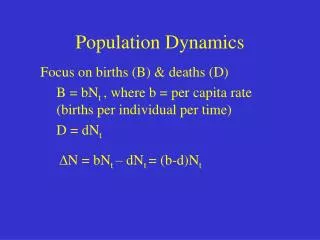
Population Dynamics • Focus on births (B) & deaths (D) • B = bNt , where b = per capita rate (births per individual per time) • D = dNt • N = bNt – dNt = (b-d)Nt
Exponential Growth • Density-independent growth models • Discrete birth intervals (Birth Pulse) • vs. • Continuous breeding (Birth Flow)
> 1 • < 1 • = 1 Nt = N0 t
Geometric Growth • When generations do not overlap, growth can be modeled geometrically. Nt = Noλt • Nt = Number of individuals at time t. • No = Initial number of individuals. • λ = Geometric rate of increase. • t = Number of time intervals or generations.
Exponential Growth • Birth Pulse Population (Geometric Growth) • e.g., woodchucks • (10 individuals to 20 indivuals) • N0 = 10, N1 = 20 • N1 = N0 , • where = growth multiplier = finite rate of increase > 1 increase < 1 decrease = 1 stable population
Exponential Growth • Birth Pulse Population • N2 = 40 = N1 • N2 = (N0 ) = N0 2 • Nt = N0 t • Nt+1 = Nt
Exponential Growth • Density-independent growth models • Discrete birth intervals (Birth Pulse) • vs. • Continuous breeding (Birth Flow)
Exponential Growth • Continuous population growth in an unlimited environment can be modeled exponentially. dN / dt = rN • Appropriate for populations with overlapping generations. • As population size (N) increases, rate of population increase (dN/dt) gets larger.
Exponential Growth • For an exponentially growing population, size at any time can be calculated as: Nt = Noert • Nt = Number individuals at time t. • N0 = Initial number of individuals. • e = Base of natural logarithms =2.718281828459 • r = Per capita rate of increase. • t = Number of time intervals.
Nt = N0ert Difference Eqn Note: λ = er
Exponential growth and change over time N = N0ert dN/dt = rN Number (N) Slope (dN/dt) Time (t) Number (N) Slope = (change in N) / (change in time) = dN / dt
ON THE MEANING OF r • rm - intrinsic rate of increase – unlimited • resourses • rmax– absolute maximal rm • - also called rc = observed r > 0 r < 0 r = 0
Intrinsic Rates of Increase • On average, small organisms have higher rates of per capita increase and more variable populations than large organisms.
Growth of a Whale Population • Pacific gray whale (Eschrichtius robustus) divided into Western and Eastern Pacific subpopulations. • Rice and Wolman estimated average annual mortality rate of 0.089 and calculated annual birth rate of 0.13. 0.13 - 0.089 = 0.041 • Gray Whale population growing at 4.1% per yr.
Growth of a Whale Population • Reilly et.al. used annual migration counts from 1967-1980 to obtain 2.5% growth rate. • Thus from 1967-1980, pattern of growth in California gray whale population fit the exponential model: Nt = Noe0.025t
What values of λ allow Population Growth Stable Population Size Population Decline What values of r allow Population Growth Stable Population Size Population Decline • λ > 1.0 • r > 0 • λ = 1.0 • r = 0 • λ < 1.0 • r < 0
Logistic Population Growth • As resources are depleted, population growth rate slows and eventually stops • Sigmoid (S-shaped) population growth curve • Carrying capacity (K): number of individuals of a population the environment can support • Finite amount of resources can only support a finite number of individuals
Logistic Population Growth dN / dt = rN dN/dt = rN(1-N/K) • r = per capita rate of increase • When N nears K, the right side of the equation nears zero • As population size increases, logistic growth rate becomes a small fraction of growth rate • Highest when N=K/2 • N/K = Environmental resistance
Limits to Population Growth • Environment limits population growth by altering birth and death rates • Density-dependent factors • Disease, Resource competition • Density-independent factors • Natural disasters
Logistic Population Model Nt = 2, R = 0.15, K = 450 A. Discrete equation - Built in time lag = 1 - Nt+1 depends on Nt
I. Logistic Population Model B. Density Dependence
Logistic Population ModelC. Assumptions • No immigration or emigration • No age or stage structure to influence births and deaths • No genetic structure to influence births and deaths • No time lags in continuous model
K Logistic Population ModelC. Assumptions • Linear relationship of per capita growth rate and population size (linear DD)
Logistic Population ModelC. Assumptions • Linear relationship of per capita growth rate and population size (linear DD) • Constant carrying capacity – availability of resources is constant in time and space • Reality?
I. Logistic Population Model Discrete equation Nt = 2, r = 1.9, K = 450 Damped Oscillations r <2.0
I. Logistic Population Model Discrete equation Nt = 2, r = 2.5, K = 450 Stable Limit Cycles 2.0 < r < 2.57 * K = midpoint
I. Logistic Population Model Discrete equation Nt = 2, r = 2.9, K = 450 • Chaos • r > 2.57 • Not random • change • Due to DD • feedback and time • lag in model
Underpopulation or Allee Effect • Opposite type of DD • population size down and population growth down b=d b=d d Vital rate b b<d r<0 N* K N
Review of Logistic Population ModelD. Deterministic vs. Stochastic Models Nt = 1, r = 2, K = 100 * Parameters set deterministic behavior same
Nt = 1, r = 0.15, SD = 0.1; K = 100, SD = 20 Review of Logistic Population ModelD. Deterministic vs. Stochastic Models * Stochastic model, r and K change at random each time step
Nt = 1, r = 0.15, SD = 0.1; K = 100, SD = 20 Review of Logistic Population ModelD. Deterministic vs. Stochastic Models * Stochastic model
Nt = 1, r = 0.15, SD = 0.1; K = 100, SD = 20 Review of Logistic Population ModelD. Deterministic vs. Stochastic Models * Stochastic model
Environmental StochasticityA. Defined • Unpredictable change in environment occurring in time & space • Random “good” or “bad” years in terms of changes in r and/or K • Random variation in environmental conditions in separate populations • Catastrophes = extreme form of environmental variation such as floods, fires, droughts • High variability can lead to dramatic fluctuations in populations, perhaps leading to extinction
Environmental StochasticityA. Defined • Unpredictable change in environment occurring in time & space • Random “good” or “bad” years in terms of changes in r and/or K • Random variation in environmental conditions in separate populations • Catastrophes = extreme form of environmental variation such as floods, fires, droughts • High variability can lead to dramatic fluctuations in populations, perhaps leading to extinction
Environmental StochasticityA. Defined • Unpredictable change in environment occurring in time & space • Random “good” or “bad” years in terms of changes in r and/or K • Random variation in environmental conditions in separate populations • Catastrophes = extreme form of environmental variation such as floods, fires, droughts • High variability can lead to dramatic fluctuations in populations, perhaps leading to extinction
Environmental StochasiticityB. Examples – variable fecundity Relation Dec-Apr rainfall and number of juvenile California quail per adult (Botsford et al. 1988 in Akcakaya et al. 1999)
Environmental StochasiticityB. Examples - variable survivorship Relation total rainfall pre-nesting and proportion of Scrub Jay nests to fledge (Woolfenden and Fitzpatrik 1984 in Akcakaya et al. 1999)
Environmental StochasiticityB. Examples – variable rate of increase Muskox population on Nunivak Island, 1947-1964 (Akcakaya et al. 1999)