Spatial locality
( m-k-n ) bits. k bits. n -bit Block Offset. Byte Address. Block Address. m -bit Address. Tag. Index. 0000 0001 0010 0011 0100 0101 0110 0111 1000 1001 1010 1011 1100 1101 1110 1111. 0 1 2 3 4 5 6 7. Index. 0 1 2 3. Spatial locality. Caches load multiple

Spatial locality
E N D
Presentation Transcript
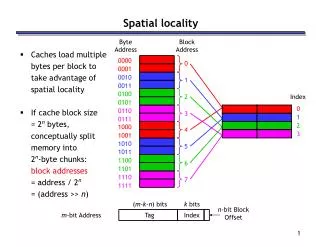
(m-k-n) bits k bits n-bit Block Offset Byte Address Block Address m-bit Address Tag Index 0000 0001 0010 0011 0100 0101 0110 0111 1000 1001 1010 1011 1100 1101 1110 1111 0 1 2 3 4 5 6 7 Index 0 1 2 3 Spatial locality • Caches load multiple bytes per block to take advantage of spatial locality • If cache block size = 2n bytes, conceptually split memory into 2n-byte chunks: block addresses = address / 2n = (address >> n)
How big is the cache? Byte-addressable machine, 16-bit addresses, cache details: • direct-mapped • block size = one byte • index = 5 least significant bits Two questions: • How many blocks does the cache hold? • How many bits of storage are required to build the cache (data plus all overhead including tags, etc.)?
Memory Address 0000 0001 0010 0011 0100 0101 0110 0111 1000 1001 1010 1011 1100 1101 1110 1111 Index 00 01 10 11 Disadvantage of direct mapping • The direct-mapped cache is easy: indices and offsets can be computed with bit operators or simple arithmetic, because each memory address belongs in exactly one block • However, this isn’t really flexible. If a program uses addresses 2, 6, 2, 6, 2, ..., then each access will result in a cache miss and a load into cache block 2 • This cache has four blocks, but direct mapping might not let us use all of them • This can result in more misses than we might like
A fully associative cache • A fully associative cache permits data to be stored in any cache block, instead of forcing each memory address into one particular block • when data is fetched from memory, it can be placed in any unused block of the cache • this way we’ll never have a conflict between two or more memory addresses which map to a single cache block • In the previous example, we might put memory address 2 in cache block 2, and address 6 in block 3. Then subsequent repeated accesses to 2 and 6 would all be hits instead of misses. • If all the blocks are already in use, it’s usually best to replace the least recently used one, assuming that if it hasn’t used it in a while, it won’t be needed again anytime soon.
Index Valid Tag (32 bits) Data Address (32 bits) ... ... ... 32 Tag Hit = = = The price of full associativity • However, a fully associative cache is expensive to implement. • Because there is no index field in the address anymore, the entire address must be used as the tag, increasing the total cache size. • Data could be anywhere in the cache, so we must check the tag of every cache block. That’s a lot of comparators!
Set associativity • An intermediate possibility is a set-associative cache • The cache is divided into groups of blocks, called sets • Each memory address maps to exactly one set in the cache, but data may be placed in any block within that set • If each set has 2x blocks, the cache is an 2x-way associative cache • Here are several possible organizations of an eight-block cache 1-way associativity 8 sets, 1 block each 2-way associativity 4 sets, 2 blocks each Set Set 0 1 2 3 0 1 2 3 4 5 6 7 4-way associativity 2 sets, 4 blocks each Set 0 1
Index V Tag Data Address Data ... 110 ... ... 1101 0110 ... 1 11010 42803 42803 Mem[1101 0110] = 21763 Index V Tag Data Address Data ... 1101 0110 ... ... 110 ... 1 11010 21763 42803 Writing to a cache • Writing to a cache raises several additional issues • First, let’s assume that the address we want to write to is already loaded in the cache. We’ll assume a simple direct-mapped cache: • If we write a new value to that address, we can store the new data in the cache, and avoid an expensive main memory access [but inconsistent] HUGE problem in multiprocessors
Mem[1101 0110] = 21763 Index V Tag Data Address Data ... 110 ... ... 1101 0110 ... 1 11010 21763 21763 Write-through caches • A write-through cache solves the inconsistency problem by forcing all writes to update both the cache and the main memory • This is simple to implement and keeps the cache and memory consistent • Why is this not so good?
Write-back caches • In a write-back cache, the memory is not updated until the cache block needs to be replaced (e.g., when loading data into a full cache set) • For example, we might write some data to the cache at first, leaving it inconsistent with the main memory as shown before • The cache block is marked “dirty” to indicate this inconsistency • Subsequent reads to the same memory address will be serviced by the cache, which contains the correct, updated data Mem[1101 0110] = 21763 Index V Dirty Tag Data Address Data ... 110 ... 1000 1110 1101 0110 ... 1225 1 1 11010 21763 42803
Dirty V 1 1 Dirty V 1 0 Finishing the write back • We don’t need to store the new value back to main memory unless the cache block gets replaced • E.g. on a read from Mem[1000 1110], which maps to the same cache block, the modified cache contents will first be written to main memory • Only then can the cache block be replaced with data from address 142 Tag Data Address Data Index 1000 1110 1101 0110 ... 1225 ... 110 ... 11010 21763 21763 Tag Data Address Data Index 1000 1110 1101 0110 ... 1225 ... 110 ... 10001 1225 21763
Index V Tag Data Address Data ... 110 ... ... 1101 0110 ... 1 00010 123456 6378 Write misses • A second scenario is if we try to write to an address that is not already contained in the cache; this is called a write miss • Let’s say we want to store 21763 into Mem[1101 0110] but we find that address is not currently in the cache • When we update Mem[1101 0110], should we also load it into the cache?
Mem[1101 0110] = 21763 Address Data Index V Tag Data ... 1101 0110 ... ... 110 ... 21763 1 00010 123456 Write around caches (a.k.a. write-no-allocate) • With a write around policy, the write operation goes directly to main memory without affecting the cache • This is good when data is written but not immediately used again, in which case there’s no point to load it into the cache yet for (int i = 0; i < SIZE; i++) a[i] = i;
Mem[214] = 21763 Index V Tag Data Address Data ... 110 ... ... 1101 0110 ... 1 11010 21763 21763 Allocate on write • An allocate on write strategy would instead load the newly written data into the cache • If that data is needed again soon, it will be available in the cache
On a write-allocate cache this would be a hit Which is it? • Given the following trace of accesses, can you determine whether the cache is write-allocate or write-no-allocate? • Assume A and B are distinct, and can be in the cache simultaneously. Miss Load A Miss Store B Hit Store A Hit Load A Miss Load B Hit Load B Hit Load A Answer: Write-no-allocate
CPU A little static RAM (cache) Lots of dynamic RAM Memory System Performance • To examine the performance of a memory system, we need to focus on a couple of important factors. • How long does it take to send data from the cache to the CPU? • How long does it take to copy data from memory into the cache? • How often do we have to access main memory? • There are names for all of these variables. • The hit time is how long it takes data to be sent from the cache to the processor. This is usually fast, on the order of 1-3 clock cycles. • The miss penalty is the time to copy data from main memory to the cache. This often requires dozens of clock cycles (at least). • The miss rate is the percentage of misses.
Average memory access time • The average memory access time, or AMAT, can then be computed AMAT = Hit time + (Miss rate x Miss penalty) This is just averaging the amount of time for cache hits and the amount of time for cache misses • How can we improve the average memory access time of a system? • Obviously, a lower AMAT is better • Miss penalties are usually much greater than hit times, so the best way to lower AMAT is to reduce the miss penaltyor the miss rate • However, AMAT should only be used as a general guideline. Remember that execution time is still the best performance metric.
Performance example • Assume that 33% of the instructions in a program are data accesses. The cache hit ratio is 97% and the hit time is one cycle, but the miss penalty is 20 cycles: • To make AMAT smaller, we can decrease the miss rate • e.g. make the cache larger, add more associativity • but larger/more complex longer hit time! • Alternate approach: decrease the miss penalty • BIG idea: a big, slow cache is still faster than RAM! • Modern processors have at least two cache levels • too many levels introduces other problems (keeping data consistent, communicating across levels)
Main Memory L2 cache CPU L1 cache Opteron Vital Statistics • L1 Caches: Instruction & Data • 64 kB • 64 byte blocks • 2-way set associative • 2 cycle access time • L2 Cache: • 1 MB • 64 byte blocks • 4-way set associative • 16 cycle access time (total, not just miss penalty) • Memory • 200+ cycle access time
12% 9% Miss rate 6% 3% 0% One-way Two-way Four-way Eight-way Associativity Associativity tradeoffs and miss rates • Higher associativity means more complex hardware • But a highly-associative cache will also exhibit a lower miss rate • Each set has more blocks, so there’s less chance of a conflict between two addresses which both belong in the same set • Overall, this will reduce AMAT and memory stall cycles • Figure from the textbook shows the miss rates decreasing as the associativity increases
15% 12% 9% 1 KB Miss rate 2 KB 4 KB 6% 8 KB 3% 0% One-way Two-way Four-way Eight-way Associativity Cache size and miss rates • The cache size also has a significant impact on performance • The larger a cache is, the less chance there will be of a conflict • Again this means the miss rate decreases, so the AMAT and number of memory stall cycles also decrease • Miss rate as a function of both the cache size and its associativity
40% 35% 30% 1 KB 25% 8 KB 20% Miss rate 16 KB 64 KB 15% 10% 5% 0% 4 16 64 256 Block size (bytes) Block size and miss rates • Finally, miss rates relative to the block size and overall cache size • Smaller blocks do not take maximum advantage of spatial locality • But if blocks are too large, there will be fewer blocks available, and more potential misses due to conflicts