Download
1 / 40
420 likes | 866 Views
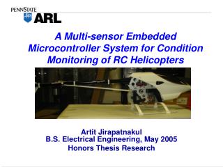
A Multi-sensor Embedded Microcontroller System for Condition Monitoring of RC Helicopters. Artit Jirapatnakul B.S. Electrical Engineering, May 2005 Honors Thesis Research. System Capabilities. Communicate with sensors IMU: Crossbow IMU400-CC GPS: Novatel Superstar II

E N D
A Multi-sensor Embedded Microcontroller System for Condition Monitoring of RC Helicopters Artit JirapatnakulB.S. Electrical Engineering, May 2005 Honors Thesis Research
System Capabilities • Communicate with sensors • IMU: Crossbow IMU400-CC • GPS: Novatel Superstar II • Compass: Honeywell HMR3100 • Data processing • Reliable data transmission to computer • Visualization in graphical interface
Crossbow IMU400CC Linear acceleration along three orthogonal axes Rotational rates along three orthogonal axes Connected via RS232 at 38.4kbps Novatel Superstar II Latitude and Longitude Velocity Altitude Time and Date Connected via RS232 at 9.6kbps Honeywell HMR3100 Measures heading Connected via RS232 at 9.6kbps Sensors
Compass IMU GPS Sensors Sensors mounted in plastic containment unit
PIC18F8720 16-bit RISC CPU Up to 10MIPS 3840 bytes RAM dsPIC30F6014 16-bit RISC CPU with DSP Up to 30MIPS 8192 bytes RAM Microcontrollers
System Design • Several processing boards are used • Advantages • Allows greater number of sensors to be used • Boards can be located closer to sensors • Distributed processing • Disadvantages • Slightly greater complexity
System Diagram using PIC18s 38.4kbps IMU 57.6kbps Slave PIC* 9.6kbps 57.6kbps Compass Master PIC 9.6kbps GPS * Can also be used with dsPIC instead
System Setup using dsPIC Laptop for visualization Sensor box dsPIC development board System setup with dsPIC and IMU connected to laptop
Results • Sensor monitoring with PIC18 • Can PIC18 keep up with data rate of all three sensors? • Connected IMU, GPS, and Compass to two PIC18 boards • PIC18 boards decoded sensor packets and multiplexed them
Results • Sensor monitoring with PIC18 • Communication with sensors successful • PIC18 is able to process at data rates of sensors • Graphical interface works correctly
Results • dsPIC processing of IMU data • Perform ten sample sliding window RMS calculation in real-time • Transmit unprocessed IMU data along with RMS values for three linear accelerations
Results • Statistics calculations on PIC18 Ten sample sliding window RMS calculation by PIC18 compared to calculations in MATLAB
Results • Statistics calculation on PIC18 Ten sample sliding window skew calculation performed by PIC as compared with calculations in MATLAB
Results • Statistics calculation on PIC18 Ten sample sliding window kurtosis calculation on PIC18 compared to calculation in MATLAB
Future Work • Wireless connection between system and computer • Design and fabricate small PC boards for system • Testing with additional algorithms • Actual flight testing
Multi-Sensor Fusion For Feature Tracking and Prediction Using Particle Filters Cory Smith M.S. Electrical Engineering, May 2005 Committee Members: Dr. Kenneth Jenkins – Co-advisor Dr. Amulya Garga – Co-advisor Dr. David Hall – Committee Member
Presentation Outline • Motivation and thesis focus • Theory – Kalman and particle filtering, prediction, remaining useful life (RUL) of mechanical systems • Results – simulation data and mechanical fault data collected by the Conditioned-Based Maintenance department • Decision-level fusion – theory and results • Conclusions and further research topics
Motivation • Tracking in real-world scenarios usually involves systems with non-linear models and non-Gaussian noise • Kalman filter provides the optimal solution as long as the system is linear with Gaussian noise • Particle filter does not require Gaussian noise distributions and works with both linear and non-linear models
Focus of the Thesis • Compare Kalman and particle filters with regard to their ability to track and predict features using simulated data and CBM mechanical fault data • Estimate remaining useful life (RUL) of mechanical systems • Utilize decision-level data fusion techniques to increase RUL accuracy
Kalman FilteringProcessing Steps (Gelb, 1974) Predict Forward Compute Kalman Gain Receive Measurement Update Prediction
State Vector: Transition Matrix: Measurement Vector: Process Noise Matrix: Kalman FilteringModels for Application Estimating position, velocity and acceleration Based on kinematics: Only measuring position Derivation may be found in (Bar-Shalom, 1993)
Particle FilterFundamentals • Particle filters do not rely on any assumptions regarding noise distributions or linear models • Utilizes Monte Carlo (MC) Integration to approximate the true density • Choose an initial proposal density (Ex: Gaussian) to get started, then use the prior distribution as the proposal • As the number of samples approaches infinity, the proposal density approaches the true density • The particle filter is more computationally intensive than the Kalman filter
Particle FilterProcessing Flow (Ristic, 2004) Draw Samples from Proposal Density (Predict Forward) Receive Measurement Compute Particle Weights Update Proposal
Particle FilterGraphical Representation (Doucet, 2001) Initial Proposal Density (Ex. Gaussian) Sample from Proposal Density and Predict Forward True Underlying Posterior Density Take measurement, compute likelihoods, and weight particles accordingly. This becomes the new proposal density for k+1.
Particle FilterDegeneracy Phenomenon • After a few iterations, all but one particle will contain negligible weight. Solution: Resample (Ristic, 2004) • Refine proposal density by sampling from the particles with high weights and discarding those with negligible weights. • This will focus on “important” areas of the distribution giving it more “definition” to resemble the true underlying distribution
Particle FilterResampling (Ristic, 2004) Resample from “important areas” of the estimated density New normalized particles for k+1
Prediction • The Kalman and particle filters may be used to estimate the state without any measurement updates • The prediction relies only on the prediction equations for each filter: (KF) (PF) • The state transition and process noise matrices become a function of the time interval since the last measurement:
Remaining Useful Life (RUL) • RUL is the amount of time left before a system reaches mechanical failure
Feature Plot Tracking Error Third-Order Simulation Third-order simulation data was generated using the model: where a is zero-mean Gaussian noise ~ N(0,0.2)
Proc. Noise = 0.9 Proc. Noise = 0.009 Third-Order SimulationParticle Paths • With the high process noise many particles are discarded during resampling • By lowering the process noise, more particles have sufficient weight
Computational Comparison • Kalman filter is O(2d3) dominated by the covariance update • Particle filter is O(Nd2) from individual particle propagation (Gustafsson, 2002) • The computation time for both filters was computed using cputime in Matlab • Plot shows that increasing the number of particles increases the computational costs as expected
H-60 Intermediate Gearbox (IGB) 3 Separate Seeded Fault Run to Failure Tests EDM Notch Initiated at Input Pinion Tooth Root (EDM: Electrical Discharge Machine) 2 Accelerometers (100kHz sampling) Source: NAVAIR 4.4.2 Patuxent River Naval Air Station
References • Bar-Shalom, Y., Li, X.-R., Estimation and Tracking: Principles, Techniques, and Software, Boston, MA, Artech House, 1993. • Cleveland, W. S., “Robust Locally Weighted Regression and Smoothing Scatterplots,” Journal of the American Statistical Association, Vol. 74, No. 368,Dec. 1979, pp. 829-836. • Doucet, A., Freitas, N., Gordon, N., Sequential Monte Carlo Methods in Practice,New York, NY, Springer-Verlag, 2001. • Erdley, J., “Data Fusion for Improved Machinery Fault Classification,” M.S. Thesis in Electrical Engineering, The Pennsylvania State University, University Park, PA, May., 1997 • Gelb, A., and technical staff of The Analytic Sciences Corportation, Applied Optimal Estimation, The M.I.T. Press, Cambridge, Massachusetts, and London, England,1974. • Gustafsson, F., Gunnarsson, F., Bergman, N., Forssell, U., Jansson, J., Karlsson, R., and Nordlund, P.-J., “Particle Filters for Position, Navigation, and Tracking,” IEEE Transactions on Signal Processing, Vol. 50, No. 2, Feb. 2002, pp. 425-237. • McClintic, K. T., “Feature Prediction and Tracking for Monitoring the Condition of Complex Mechanical Systems,” M.S. Thesis in Acoustics, The Pennsylvania State University, University Park, PA, Dec., 1998 • Ristic, B., Arulampalam, S., Gordon, N., Beyond the Kalman Filter, Boston, MA, Artech House, 2004.
Time = 50 Hrs. N=100, Proc. Noise = 0.009 N=100, Proc. Noise = 0.9 N=500, Proc. Noise = 0.009 N=500, Proc. Noise = 0.9 N=1000, Proc. Noise = 0.009 N=1000, Proc. Noise = 0.9 Third-Order SimulationParticle Distributions