Supply and Demand
Supply and Demand. Overheads. Equilibrium. Equilibrium is defined a state of rest; a situation that, one achieved, will not change, unless some external factor, previously held constant, changes. Market Equilibrium. A market is said to be in equilibrium

Supply and Demand
E N D
Presentation Transcript
Supply and Demand Overheads
Equilibrium Equilibrium is defined a state of rest; a situation that, one achieved, will not change, unless some external factor, previously held constant, changes.
Market Equilibrium A market is said to be in equilibrium if the price in the market is such that the quantity supplied (QS) in the market and the quantity demanded (QD) in the market are equal.
Supply = Demand D0 S0 3333.33 6666.66 Demand and Supply of Hamburger Patties 3.5 Price 3 2.5 2 1.5 1 0.5 0 0 2000 4000 6000 8000 10000 12000 Quantity
Quantity Quantity Price (per lb) supplied demanded 0.3 1000 9800 0.60 2000 8600 0.90 3000 7400 1.20 4000 6200 1.50 5000 5000 1.80 6000 3800 2.10 7000 2600 2.40 8000 1400 2.50 9000 200
Excess supply and excess demand Excess supply At a given price, the excess of the quantity supplied over the quantity demand is called the excess supply. Excess supply = QS (P) - QD (P)
Quantity Quantity Price (per lb) supplied demanded 0.3 1000 9800 0.60 2000 8600 0.90 3000 7400 1.20 4000 6200 1.50 5000 5000 1.80 6000 3800 2.10 7000 2600 2.40 8000 1400 2.50 9000 200 At a price of $2.10, excess supply (QS (P) - QD (P) ) is given by 7,000 - 2,600 = 4,400
Quantity Quantity Price (per lb) supplied demanded 0.3 1000 9800 0.60 2000 8600 0.90 3000 7400 1.20 4000 6200 1.50 5000 5000 1.80 6000 3800 2.10 7000 2600 2.40 8000 1400 2.50 9000 200 At a price of $1.20, excess supply (QS (P) - QD (P) ) is given by 4,000 - 6,200 = -2,200
Excess demand At a given price, the excess of the quantity demanded over the quantity supplied is called the excess demand. Excess Demand = QD (P) - QS (P)
Quantity Quantity Price (per lb) supplied demanded 0.3 1000 9800 0.60 2000 8600 0.90 3000 7400 1.20 4000 6200 1.50 5000 5000 1.80 6000 3800 2.10 7000 2600 2.40 8000 1400 2.50 9000 200 At a price of $0.90, excess demand (QD (P) - QS (P) ) is given by 7,400 - 3,000 = 4,400
Quantity Quantity Price (per lb) supplied demanded 0.3 1000 9800 0.60 2000 8600 0.90 3000 7400 1.20 4000 6200 1.50 5000 5000 1.80 6000 3800 2.10 7000 2600 2.40 8000 1400 2.50 9000 200 At a price of $2.10, excess demand (QD (P) - QS (P) )is given by 2,600 - 7,000 = -4,400
Market Equilibrium A market is in equilibrium when the price is such that the quantity supplied is equal to quantity demanded. A market is in equilibrium when the price is such that excess supply equals excess demand equals zero.
Excess supply and excess demand and price pressure When the quantity demanded in the market exceeds the quantity supplied at a given price, QD (P) > QS (P) there is excess demand, and the price will tend to rise.
Excess demand and excess supply and price pressure When the price in the market rises, quantity demanded falls & quantity supplied rises until an equilibrium is reached at which quantity demanded equals quantity supplied.
The process of price rising so that excess demand falls to zero is called price rationing
QS (P) >QD (P) Supply = Demand D0 S0 Graphical analysis of excess supply 3.5 Price 3 Price Falls 2.5 2 1.5 1 0.5 0 0 2000 4000 6000 8000 10000 12000 Quantity
Supply = Demand D0 S0 QD (P) > QS (P) Graphical analysis of excess demand 3.5 Price Price Rises 3 2.5 2 1.5 1 0.5 0 0 2000 4000 6000 8000 10000 12000 Quantity
Algebraic analysis of supply and demand Equilibrium Supply = Demand To find an equilibrium in a market: 1. Set supply equal to demand and solve for P. 2. Substitute P in the supply and demand equations to get the quantities.
Example Demand Equation QD = 20 - 2P
D0 Demand QD = 20 - 2P 14 Price 12 10 8 6 4 2 0 0 2 4 6 8 10 12 14 16 18 20 22 24 Quantity
Example Supply Equation QS -4 + 2P
S0 Supply QS -4 + 2P 14 Price 12 10 8 6 4 2 0 0 2 4 6 8 10 12 14 16 18 20 22 24 Quantity
D0 S0 Demand and Supply QD = 20 - 2P QS -4 + 2P 14 Price 12 10 8 6 4 2 0 0 2 4 6 8 10 12 14 16 18 20 22 24 Quantity
Example Calculation Set supply equal to demand and solve the equation for P. QD = 20 - 2P = -4 + 2P = QS 20 - 2P = -4 + 2P +4 + 4 • 24 - 2P = 2P +2P +2P QD = 20 - 2P = 20 – 2(6) = 8 24 = 4P • 24 = 4P • 4 4 • 6 = P
Some notes on solving equations We get equivalent equations if on both sides of the equality sign we do the following: a. add the same number b. subtract the same number c. multiply by the same number 0 d. divide by the same number 0.
Comparative Statics or What happens when things change Demand Shifts Increases in demand (shifts to the right) will increase the equilibrium price and quantity. Decreases in demand (shifts to the left) will decrease the equilibrium price and quantity.
S0 D0 D1 D2 Changes in Demand 16 Price 14 12 10 8 6 4 2 0 0 5 10 15 20 25 Quantity
Supply Shifts Increases in supply (shifts to the right) will decrease the equilibrium price and increase the equilibrium quantity. Decreases in supply (shifts to the left) will increase the equilibrium price and decrease the equilibrium quantity.
D0 S0 S2 S1 Changes in Supply Price 14 12 10 8 6 4 2 0 0 5 10 15 20 Quantity
Price Ceilings A price ceiling occurs when some outside force sets a price for the market that is below the equilibrium price. When quantity supplied & quantity demanded differ, the short side of the market — whichever of the two quantities is less — will prevail.
Supply Demand D0 S0 QD (P) > QS (P) Price Ceiling 3.5 Price Queuing 3 2.5 2 1.5 1 0.5 0 0 2000 4000 6000 8000 10000 12000 Quantity
Queuing Shortages The results: A black market
Price Floors A price floor occurs when some outside force sets a price for the market that is above the equilibrium price. When quantity supplied & quantity demanded differ, the short side of the market — whichever of the two quantities is less — will prevail.
QS (P) >QD (P) Supply Demand D0 S0 Price Floor 3.5 Price Excess Supply 3 2.5 2 1.5 1 0.5 0 0 2000 4000 6000 8000 10000 12000 Quantity
The results: Excess supply Unemployment