Forecasting, continued
Forecasting, continued. What did you learn from the forecasting exercise? Are you making the spreadsheet do the work for you? How does the projected growth compare to SGR & IGR, and to economic limitations? Do the figures make sense?

Forecasting, continued
E N D
Presentation Transcript
Forecasting, continued What did you learn from the forecasting exercise? Are you making the spreadsheet do the work for you? How does the projected growth compare to SGR & IGR, and to economic limitations? Do the figures make sense? How does this connect to your knowledge of the company’s strategy?
Assumptions What assumptions are we making about the subject company? How can we test each? What segments for sales are you using? How are you attributing growth to volume & price? What is the subject company’s relationship between sales & assets? What about costs of raw materials?
Valuation Value = Debt Value + Equity Value Equity Value / Shares Outstanding = “Correct” Price per Share (Intrinsic Value per Share) Context & perspective come from comparables and other less robust methods Publicly traded company can be declared to be “overvalued” or “undervalued”
Expected Cash Flows Forecast, then Recast Start by predicting what is likely to be published on the financial statements. After that, recast the figures to better reflect the economic realities for operating leases, R&D (if applicable) and sustainability of operating cash flows. Compute cash flows using more than one formula to ensure you have found all the issues in your figures.
Measuring Cash Flows To go from reported to actual earnings we may have to: • Update earnings & data to the date of interest • Make corrections from Accounting Earnings • Adjust for One-Time and Non-recurring Charges
One-Time and Non-recurring Charges Assume that you are valuing a firm that is reporting a loss of $ 500 million, due to a one-time charge of $ 1 billion. What is the earnings you would use in your valuation? A loss of $ 500 million A profit of $ 500 million Would your answer be any different if the firm had reported one-time losses like these once every five years? Yes No
Correcting Accounting Earnings COGS Adjustment: Inventory costs are associated with particular goods using one of several formulas, including specific identification, last-in first-out (LIFO), first-in first-out (FIFO), or average cost. This may affect the value of a firm compared to the accounting information presented. The Operating Lease Adjustment: While accounting convention treats operating leases as operating expenses, they are really financial expenses and need to be reclassified as such. This has no effect on equity earnings but does change the operating earnings The R & D Adjustment: Since R&D is a capital expenditure (rather than an operating expense), the operating income has to be adjusted to reflect its treatment (only if there is significant intellectual property).
Inventory Valuation There are three basis approaches to valuing inventory that are allowed by GAAP(a) First-in, First-out (FIFO): Under FIFO, the cost of goods sold is based upon the cost of material bought earliest in the period, while the cost of inventory is based upon the cost of material bought later in the year. This results in inventory being valued close to current replacement cost. During periods of inflation, the use of FIFO will result in the lowest estimate of cost of goods sold among the three approaches, and the highest net income.(b) Last-in, First-out (LIFO): Under LIFO, the cost of goods sold is based upon the cost of material bought towards the end of the period, resulting in costs that closely approximate current costs. The inventory, however, is valued on the basis of the cost of materials bought earlier in the year. During periods of inflation, the use of LIFO will result in the highest estimate of cost of goods sold among the three approaches, and the lowest net income.(c) Weighted Average: Under the weighted average approach, both inventory and the cost of goods sold are based upon the average cost of all units bought during the period. When inventory turns over rapidly this approach will more closely resemble FIFO than LIFO.
Firms often adopt the LIFO approach for the tax benefits during periods of high inflation, and studies indicate that firms with the following characteristics are more likely to adopt LIFO - rising prices for raw materials and labor, more variable inventory growth, an absence of other tax loss carry forwards, and large size. When firms switch from FIFO to LIFO in valuing inventory, there is likely to be a drop in net income and a concurrent increase in cash flows (because of the tax savings). The reverse will apply when firms switch from LIFO to FIFO. Given the income and cash flow effects of inventory valuation methods, it is often difficult to compare firms that use different methods. There is, however, one way of adjusting for these differences. Firms that choose to use the LIFO approach to value inventories have to specify in a footnote the difference in inventory valuation between FIFO and LIFO, and this difference is termed the LIFO reserve. This can be used to adjust the beginning and ending inventories, and consequently the cost of goods sold, and to restate income based upon FIFO valuation. Inventory Valuation
Dealing with Operating Lease Expenses Operating Lease Expenses are treated as operating expenses in computing operating income. In reality, operating lease expenses should be treated as financing expenses, with the following adjustments to earnings and capital: Debt Value of Operating Leases = PV of Operating Lease Expenses at the pre-tax cost of debt Adjusted Operating Earnings Adjusted Operating Earnings = Operating Earnings + Operating Lease Expenses - Depreciation on Leased Asset As an approximation, this works: Adjusted Operating Earnings = Operating Earnings + Pre-tax cost of Debt * PV of Operating Leases.
Effects of Capitalizing Operating Leases Debt : will increase, leading to an increase in debt ratios used in the cost of capital and levered beta calculation Operating income: will increase, since operating leases will now be before the imputed interest on the operating lease expense Net income: will be unaffected since it is after both operating and financial expenses anyway Return on Capital will generally decrease since the increase in operating income will be proportionately lower than the increase in book capital invested
Dealing with Operating Leases In 1998, Home Depot did not carry much in terms of traditional debt on its balance sheet. However, it did have significant operating leases. When doing firm valuation, these operating leases have to be treated as debt. This, in turn, will mean that operating income has to get restated.
Operating Leases at Home Depot in 1998 The pre-tax cost of debt at the Home Depot is 5.80% Year Commitment Present Value 1 $294.00 $277.88 2 $291.00 $259.97 3 $264.00 $222.92 4 $245.00 $195.53 5 $236.00 $178.03 6 and beyond $2700.00 $1,513.37 Debt Value of leases = $2,647.70
Operating Leases at Home Depot in 1998 The pre-tax cost of debt at the Home Depot is 5.80% Year Commitment Present Value 1 $294.00 $277.88 2 $291.00 $259.97 3 $264.00 $222.92 4 $245.00 $195.53 5 $236.00 $178.03 6 and beyond $2700.00 $1,513.37 Debt Value of leases = $2,647.70 Average = 266 PV of 270/yr for 10 yrs 2700 / 266 =~10 yrs 2700 / 10 = 270/yr for years 6-15
Other Adjustments from Op. Leases Operating Lease Operating Lease Expensed converted to Debt EBIT $ 2,661mil $ 2,815 mil EBIT (1-t) $1,730 mil $1,829 mil Debt $1,433 mil $ 4,081 mil What else?
Capitalizing R&D Expenses Accounting standards require us to consider R&D as an operating expense even though it is designed to generate future growth. It is more logical to treat it as capital expenditures. What’s the difference between R&D and NPD? Not all so-called R&D produces assets. If it does, it should be capitalized To capitalize R&D, Specify an amortizable life for R&D (2 - 10 years) Collect past R&D expenses for as long as the amortizable life Sum up the unamortized R&D over the period. (Thus, if the amortizable life is 5 years, the research asset can be obtained by adding up 1/5th of the R&D expense from five years ago, 2/5th of the R&D expense from four years ago...:
Capitalizing R&D Expenses: Cisco R & D was assumed to have a 5-year life. (all figures as of 1999 data) Year R&D Expense Unamortized portion Amortization this year 1999 1594.00 1.00 1594.00 1998 1026.00 0.80 820.80 $205.20 1997 698.00 0.60 418.80 $139.60 1996 399.00 0.40 159.60 $79.80 1995 211.00 0.20 42.20 $42.20 1994 89.00 0.00 0.00 $17.80 Total $ 3,035.40 $ 484.60 Value of research asset = $ 3,035.4 million Amortization of research asset in 1998 = $ 484.6 million Adjustment to Operating Income = $ 1,594 million - 484.6 million = 1,109.4 million
The Effect of Capitalizing R&D Operating Income will generally increase, though it depends upon whether R&D is growing or not. If it is flat, there will be no effect since the amortization will offset the R&D added back. The faster R&D is growing the more operating income will be affected. Net income will increase proportionately, depending again upon how fast R&D is growing Book value of equity (and capital) will increase by the capitalized Research asset Capital expenditures will increase by the amount of R&D; Depreciation will increase by the amortization of the research asset; For all firms, the net cap ex will increase by the same amount as the after-tax operating income.
Net Capital Expenditures Net capital expenditures represent the difference between capital expenditures and depreciation. Depreciation is a cash inflow that pays for some or a lot (or sometimes all of) the capital expenditures. In general, the net capital expenditures will be a function of how fast a firm is growing or expecting to grow. High growth firms will have much higher net capital expenditures than low growth firms. Assumptions about net capital expenditures can therefore never be made independently of assumptions about growth in the future.
Capital expenditures should include Research and development expenses, once they have been re-categorized as capital expenses. The adjusted net cap ex will be Adjusted Net Capital Expenditures = Net Capital Expenditures + Current year’s R&D expenses - Amortization of Research Asset Acquisitions of other firms, since these are like capital expenditures. The adjusted net cap ex will be Adjusted Net Cap Ex = Net Capital Expenditures + Acquisitions of other firms - Amortization of such acquisitions Two caveats: 1. Most firms do not do acquisitions every year. Hence, a normalized measure of acquisitions (looking at an average over time) should be used 2. The best place to find acquisitions is in the statement of cash flows, usually categorized under other investment activities
Cisco’s Acquisitions: 1999 Acquired Method of Acquisition Price Paid GeoTel Pooling $1,344 Fibex Pooling $318 Sentient Pooling $103 American Internet Purchase $58 Summa Four Purchase $129 Clarity Wireless Purchase $153 Selsius Systems Purchase $134 PipeLinks Purchase $118 Amteva Tech Purchase $159 $2,516
Cisco’s Net Capital Expenditures in 1999 Cap Expenditures (from statement of CF) = $ 584 mil - Depreciation (from statement of CF) = $ 486 mil Net Cap Ex (from statement of CF) = $ 98 mil + R & D expense = $ 1,594 mil - Amortization of R&D = $ 485 mil + Acquisitions = $ 2,516 mil Adjusted Net Capital Expenditures = $3,723 mil (Amortization was included in the depreciation number)
Working Capital Investments In accounting terms, the working capital is the difference between current assets (inventory, cash and accounts receivable) and current liabilities (accounts payables, short term debt and debt due within the next year) A cleaner definition of working capital from a cash flow perspective is the difference between non-cash current assets (inventory and accounts receivable) and non-debt current liabilities (accounts payable) Any investment in this measure of working capital ties up cash. Therefore, any increases in working capital will reduce cash flows in that period. When forecasting future growth, it is important to forecast the effects of such growth on working capital needs, and building these effects into the cash flows.