Estimation and Hypothesis Testing

1. Estimation and Hypothesis Testing

2. The Investment Decision • What would you like to know? • What will be the return on my investment? • Not possible • PDF for return • Assume the normal PDF • Use statistics to estimate E[r] and s. Use statistics to estimate the correct PDF. Can do for discrete PDF’s. For continuous PDFs, beyond the scope of this course.

3. The Game of Investing • Suppose you’re offered to play a game: • Cost: $1.25 • Flip a coin • If heads, you get $2 (return is 60%) • If tails, you get $0 (return is -100%) • Coin may be biased • Assume the true pdf for this investment is • Of course, this information is unknown!

4. The Game of Investing • You would like to know • What will the coin flip turn out to be? • Not possible • What is the PDF (probability of getting heads/tails)? • Not possible to know with certainty: need to estimate • E[r] and s • Not possible to know perfectly: need to estimate. • How to estimate? Why not flip the coin a few times?

5. Random Sample • Suppose you flip the coin 10 times and get • H, H, T, H, H, H, H, H, H, T • 8 heads, 2 tails • This is an independent random sample • A sample of observations generated by the same pdf • Independent: One outcome does not affect others • Nothing other than the pdf determines how observations are chosen. • No “cherry picking”: picking certain observations you like, and eliminating others • How do we use this information to estimate • f(heads) • E[r] • s

6. Estimators • Estimator – function of outcomes for a random sample. • An estimator is a random variable • It has it’s own PDF! • Let be an estimator of E[r] • Two important properties of estimators: • Unbiased: • Consistent: As the number of observations we observe becomes large, • Suppose we use the following rule to get our estimator of E[r]: • For any random sample, choose the first observation as our estimate of E[r]. • Call this estimator r1.

7. Estimator of E[r] • Is r1 unbiased? • For any random sample of any size, r1 is simply a random variable governed by the pdf • So E[r1]=12%=E[r] • r1 is therefore an unbiased estimator of E[r]

8. Estimator of E[r] • Is r1 consistent? • For any random sample of any size, r1 is simply a random variable governed by the pdf • So Var[r1]=0.5376 for any sample size. • r1 is therefore not a consistent estimator of E[r]

9. Estimator of E[r] • Suppose we use the following rule to get our estimator of E[r]: • For any random sample, take the average return as our estimator of E[r]. • Call this estimator .

10. Estimator of E[r] • Is unbiased? • What is ? Use stat rule #1 • is therefore an unbiased estimator of E[r]

11. Estimator of E[r] • Is consistent? • How do we find the variance of a sum of random variables? • We haven’t learned this yet, but we will later. • We can generate random samples of estimators to get some idea of the properties of their PDF. • For each outcome for an estimator, we need to generate a random sample of observations, and then compute the estimator. • Use Excel Spreadsheet (posted on course website)

12. Comment • Why do we use probability weights when calculating E[r] from a pdf, but when we estimate E[r] we just use an equally weighted average? • Given the PDF above, we should expect in any random sample to see heads 70% of the time. • Assume we draw a sample where exactly 70% are heads • 70% of the returns in the sample will be 0.60 • 30% of the returns in the sample will be -1.00 • A simple average across observations is equal to • Simple averages naturally put more weight on those outcomes which are more likely.

13. Estimator of Stdev[r] • How do we use data to estimate Stdev[r]? • Var[r]=E(r-E[r])2 = E[r2]-E[r]2 • Stdev(r)=sqrt(Var(r)) • Suppose we use the following rule to get our estimator of Stdev[r]: • Is the estimator unbiased? • Is the estimator consistent? • Use Excel spreadsheet.

14. Average • The same results apply to continuous PDFs • For a given random sample:

15. Estimates • When is the average a good estimate of E[r]? • When is our estimator for standard deviation a good estimate of Stdev[r]? • When you have a large sample of outcomes • When the PDF doesn’t change mid-sample

16. Stat Rules • Stat Rule 1.E • Let x1,…,xnbe a random sample of the random variable X. • Let y1,…,ynbe a random sample of the random variable Y. • Let zi=axi+byi, for i=1,…,n where a and b are constants. • Then • Stat Rule 2.E • Let x1,…,xnbe a random sample of the random variable X. • Let zi=axi+c, for i=1,…,n where a is a constant • Then

17. Estimated Sharpe Ratio • The Sharpe Ratio may be estimated as where we use the yield on a t-bill as a proxy for the risk-free rate.

18. Time and E[r] and Stdev[r] • E[r] and stdev[r] have a unit of time attached to them. • E[r]=10% over a year is much different than E[r]=10% over a day. • s[r]=0.16 over a year is much different than s[r]=0.16 over a day. • Let p denote a “short” time period (e.g., a month) • Let P denote a “long” time period (e.g., a year) • Let N denote the number of “short” time periods in a “long” time period (e.g., 12) • Let Ep[r] and sp[r] be the appropriate parameters over the short time period • Let EP[r] and sP[r] be the appropriate parameters over the long time period • Then to a close approximation,

19. How Good Are the Estimates? • Does the E[r] for a stock meet some pre-determined benchmark? • You can’t observe the PDF to calculate the true E[r] • Over the past 10 years, returns have been as follows: • From this you estimate E[r] to be 18.3% • Is this enough information to reject the hypothesis that the true E[r] for the PDF that generated this sample is 10%?

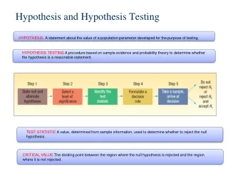
20. Hypothesis Testing • Null Hypothesis • The hypothesis to be tested • E[r]=10% • Alternative Hypothesis • E[r] ¹ 10%

21. Hypothesis Testing • c = distance of test statistic from null hypothesis that defines zone of acceptance.

22. Hypothesis Testing • Standard Practice: Choose c so that we know the probability of making a type 1 error.

23. Hypothesis Tests of the Mean • Let (X1, X2, …,Xn) be an independent random sample from anyPDF • True mean=m • True standard deviation=s • What PDF governs the outcome for the sample average? • The laws of statistics say that the sample average is approximately • Normally distributed • True mean=m • Standard Deviation= • The standard deviation of the sample average is called the “standard error”

24. Hypothesis Testing • Null Hypothesis • E[r]=10% • Alternative Hypothesis • E[r] ¹ 10% • Assuming the null is true, the sample mean is approximately normally distributed with • m=.10 • s=0.0921

25. Normal Distribution

26. Hypothesis Testing • For any normally distributed random variable, there is only a 5% probability of getting an outcome above m+1.96s or below m-1.96s. • Assuming the null is true, there is only a 5% chance of drawing a sample average above 0.10+1.96*(0.0921) =0.2805 or below 0.10-1.96*(0.0921)=-0.08052 • If the sample average is above 0.2805 or below -0.08052, we therefore conclude that it’s too unlikley (<5%) that we would observe such an outcome, given the null is true. • Hence, the null must not be true. Reject H0.

27. Hypothesis Testing

28. Hypothesis Testing The sample average we observe is 18.3% This is in the zone of acceptance. Do not reject the null hypothesis. “We cannot reject the hypothesis that the true mean is 10% with 95% Confidence.

29. Hypothesis Tests of the Mean • Example • Hypothesis: m =2% • Alternative: m¹ 2% • 100 years of stock market returns • Sample Average = 16% • Standard Deviation = 0.18 • Hence, standard error is 0.18/10 = 0.018

30. Hypothesis Tests of the Mean • c = 1.96*0.018 = 0.03528 • Assuming null hypothesis is true, too unlikely you would observe the actual sample mean. Reject the null hypothesis.

31. T-statistic