Download
1 / 38
400 likes | 611 Views
Biostatistics-Lecture 3 Estimation , confidence interval and hypothesis testing. Ruibin Xi Peking University School of Mathematical Sciences. Some Results in Probability (1). Suppose that X, Y are independent ( ) E( cX ) = ? (c is a constant) E(X+Y) = ? Var ( cX ) = ?

E N D
Biostatistics-Lecture 3Estimation, confidence interval and hypothesis testing Ruibin Xi Peking University School of Mathematical Sciences
Some Results in Probability (1) • Suppose that X, Y are independent ( ) • E(cX) = ? (c is a constant) • E(X+Y) = ? • Var(cX) = ? • Var(X+Y) = ? • Suppose are mutually independent identically distributed (i.i.d.)
Some Results in Probability (2) • The Law of Large Number (LLN) • Assume BMI follows a normal distribution with mean 32.3 and sd 6.13
Some Results in Probability (3) • The Central Limit Theorem (CLT)
Statistical Inference • Draw conclusions about a population from a sample • Two approaches • Estimation • Hypothesis testing
Estimation • Point estimation—summary statistics from sample to give an estimate of the true population parameter • The LLN implies that when n is large, these should be close to the true parameter values • These estimates are random • Confidence intervals (CI): indicate the variability of point estimates from sample to sample
Confidence interval • Assume , then (σ is known) • Confidence interval of level 95% • Repeatedly construct the confidence interval, 95% of the time, they will cover μ • In the BMI example, μ=32.3, σ=6.13, n = 20
Confidence interval • Assume , then (σ is known) • Confidence interval • Repeatedly construct the confidence interval, 95% of the time, they will cover μ • In the BMI example, μ=32.3, σ=6.13, n = 20
Confidence Interval for the Mean • Assume , then (σ is known) • Confidence interval of level 1-α
Confidence Interval for the Mean • Assume , then (σ is known) • Confidence interval of level 1-α 1-α/2
Confidence Interval for the Mean • Assume , then (σ is known) • Confidence interval of level 1-α • What if σ is unknown? • t-statistics!
Confidence Interval for the Mean • Assume , then • by the LLN. • Replace σ2 by , then • Confidence interval of level 1-α Standard error (SE)
Confidence Interval for the Mean • Assume , then • by the LLN. • Replace σ2 by , then • Confidence interval of level 1-α
Confidence Interval for the Mean • Measure serum cholesterol (血清胆固醇) in 100 adults • Construct a 95% CI for the mean serum cholesterol based on t-distribution • CI based on normal distribution
Confidence interval based on the CLT • Assume are i.i.d. random variable with population mean μ and population variance σ2 • Construct CI for μ? • From the CLT, approximately, • From the LLN, • The asymptotic CI of level 1-α is
Confidence Interval for the proportions • Telomerase • a ribonucleoproteinpolymerase • maintains telomere ends by addition of the telomere repeat TTAGGG • usually suppressed in postnatal somatic cells • Cancer cells (~90%) often have increased telomerase activity, making them immortal (e.g. HeLa cells) • A subunit of telomerase is encode by the gene TERT (telomerase reverse transcriptase)
Confidence Interval for the proportions • Huang et. al (2013) found that TERT promoter mutation is highly recurrent in human melanoma • 50 of 70 has the mutation • Construct a 95% CI for the proportion (p) of melanoma genomes that has the TERT promoter mutation • From the data above, our estimate is • The standard error is • The CI is • Note: to guarantee this approximation good, need p and 1-p ≥ 5/n
Hypothesis testing • Scientific research often start with a hypothesis • Aspirin can prevent heart attack • Imatinib can treat CML patient • TERT mutation can promote tumor progression • Collect data and perform statistical analysis to see if the data support the hypothesis or not
Steps in hypothesis testing • Step 1. state the hypothesis • Null hypothesis H0: no different, effect is zero or no improvement • Alternative hypothesis H1: some different, effect is nonzero Directionality—one-tailed or two-tailed μ<constant μ≠constant
Steps in hypothesis testing • Step 2. choose appropriate statistics • Test statistics depends on your hypothesis • Comparing two means z-test or t-test • Test independence of two categorical variables Fisher’s test or chi-square test
Steps in hypothesis testing • Step 3. Choose the level of significance—α • How much confidence do you want in decision to reject the null hypothesis • α is also thy type I error or false positive level • Typically 0.05 or 0.01
Steps in hypothesis testing • Step 4. Determine the critical value of the test statistics that must be obtained to reject the null hypothesis under the significance level • Example—two-tailed 0.05 significance level for z-test Rejection region
Steps in hypothesis testing • Step 5. Calculate the test statistic • Example: t-statistic • Step 6. Compare the test statistic to the critical value • If the test statistic is more extreme than the critical value, reject H0 DO NOT ACCEPT H1 • Otherwise, Do Not reject or Fail to reject H0 DO NOT ACCEPT H0
Steps in hypothesis testing: an example • Data Pima.tr in the MASS package • Data from Pima Indian heritage women living in USA (≥21) testing for diabetes • Question: Is the mean BMI of Pima Indian heritage women living in USA testing for diabetes is the same as the mean women BMI (26.5) • Step 1. state the hypothesis • Let μ be the mean BMI of Pima Indian heritage women living in USA • H0: μ=26.5; H1: μ≠26.5
Steps in hypothesis testing: an example • Step 2. Choose appropriate test • Two-sided t-test • Hypotheses problem μ=μ0; H1: μ≠ μ0 • Assumptions are independent, σ is unknown • Test statistic (under H0, follows tn-1) • Critical value • Check if the test is appropriate
Steps in hypothesis testing: an example • Step 2. Choose appropriate test • Two-sided t-test • Hypotheses problem μ=μ0; H1: μ≠ μ0 • Assumptions are independent, σ is unknown • Test statistic (under H0, follows tn-1) • Critical value • Check if the test is appropriate
Steps in hypothesis testing: an example • Step 3. Choose a significance level α=0.05 • Step 4. Determine the critical value • From n = 200, • Get • Step 5. Calculate the test statistic • Step 6. Compare the test statistic to the critical value • Since|t| > Ccri,0.05,we reject the null hypothesis
Steps in hypothesis testing: an example • Step 3. Choose a significance level α=0.05 • Step 4. Determine the critical value • From n = 200, • Get • Step 5. Calculate the test statistic • Step 6. Compare the test statistic to the critical value • Since|t| > Ccri,0.05,we reject the null hypothesis
P-value • Often desired to see how extreme your observed data is if the null is true • P-value • P-value • the probability that you will observe more extreme data under the null • The smallest significance level that your null would be rejected • In the previous example, P-value = P(|T|>t) = 1.3e-29
Making errors • Type I error (false positive) • Reject the null hypothesis when the null hypothesis is true • The probability of Type I error is controlled by the significance level α • Type II error (false negative) • Fail to reject the null hypothesis when the null hypothesis is false • Power = 1- probability of Type II error = 1- β • Power = P(reject H0 | H0 is false) • Which error is more serious? • Depends on the context • In the classic hypothesis testing framework, Type I error is more serious
Making Errors • Here’s an illustration of the four situations in a hypothesis test: α Power = 1-β 1-α β
Making Errors (cont.) • When H0 is false and we fail to reject it, we have made a Type II error. • We assign the letter to the probability of this mistake. • It’s harder to assess the value of because we don’t know what the value of the parameter really is. • There is no single value for --we can think of a whole collection of ’s, one for each incorrect parameter value.
Making Errors (cont.) • We could reduce for all alternative parameter values by increasing . • This would reduce but increase the chance of a Type I error. • This tension between Type I and Type II errors is inevitable. • The only way to reduce both types of errors is to collect more data. Otherwise, we just wind up trading off one kind of error against the other.
Power • When H0 is false and we reject it, we have done the right thing. • A test’s ability to detect a false hypothesis is called the power of the test. • The power of a test is the probability that it correctly rejects a false null hypothesis. • When the power is high, we can be confident that we’ve looked hard enough at the situation. • The power of a test is 1 – .
Original comparison With a larger sample size: Reducing Both Type I and Type II Error
Hypothesis test for single proportion • Kantarjian et al. (2012) studied the effect of imatinib therapy on CML patients • CML: Chronic myelogenousleukemia (慢性粒细胞性白血病) • 95% of patients have ABL-BCR gene fusion • Imatinib was introduced to target the gene fusion • Since 2001, the 8-year survival rate of CML patient in chronic phase is 87%(361/415) (with Imatinib treatment) • Before 1990, 20% • 1991-2000, 45%
Hypothesis test for single proportion • Suppose that we want to test if Imatinib can improve the 8-year survival rate • Step 1. state the hypothesis • H0: μ=0.45 vs H1: μ >0.45 (μ is the 8-year survival rate with Imatinib treatment) • Step 2. Choose appropriate test • Z-test based on the CLT • Test statistic • Follow standard normal under the null • Reject null if z > Ccrt
Hypothesis test for single proportion • Step 3. Choose the significance level α=0.01 • Step 4. Determine the critical value • Step 5. Calculate the test statistic • Step6. Compare the test statistic with the critical value, reject the null • Pvalue = 1.4e-66