Requirements for Single-Dish Holography

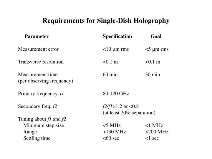
1. Requirements for Single-Dish Holography Parameter Specification Goal Measurement error <10 m rms <5 m rms Transverse resolution <0.1 m <0.1 m Measurement time 60 min 30 min (per observing frequency) Primary frequency, f1 80-120 GHz Secondary freq, f2f2/f1>1.2 or <0.8 (at least 20% separation) Tuning about f1 and f2 Minimum step size <5 MHz <1 MHz Range >130 MHz >200 MHz Settling time <60 sec <1 sec

2. Design Parameters Primary frequency 104.0 GHz Secondary frequency 78.9 GHz Tuning about each frequency >130 MHz range, <1 MHz steps Range 300 m Transmitter height above ground 50 m Transmitter height above elevation axis 43 m Nominal polarization (xmtr and rcvrs) vertical Receiver processing bandwidth 10 kHz Integrating time per measurement 12...48 msec (nominally 48 msec) Derived: Scan angle for 0.1 m resolution 2.18 deg at 78.9 GHz (1.09) 1.65 deg at 104.1 GHz (0.83) Minimum scan angle 2.29 deg due to near field geometry Transmitter beamwidth at ‑3 dB 4.6 deg (twice antenna angle@xmtr) Transmitter antenna gain 33 dB Transmitter EIRP >20 W Transmitter power to antenna >10 nW Reference antenna beamwidth, -3 dB 4.6 deg (twice scan range) Main antenna feed beamwidth, -3 dB 128 deg (-3 dB edge taper)

3. Error Budget Thermal noise <5 m rms (xmtr pwr, integ time) Feed phase pattern knowledge <5 m pk (critical) Reference antenna pattern knowledge <10 m (insensitive) Multipath interference 0.4 m (-20 dB, random phase) Frequency error 0 Near field correction error unknown RSS (except near field correction) 7.2 microns

4. Transmitter Power Calculation, inputs Assumed hardware parameters: Receiver pre‑correlation bandwidth B 10 kHz System temperature, each receiver T 3200 K Frequency f 92 GHz (l=3.26mm) Antenna diameter D 12 m j3dB = .01556o Range R 300 m Transmitter EIRP P TBD Measurement requirements: Transverse resolution D 0.1 m Surface displacement accuracy dz 5 mm Total measuring time (OTF scanning) t <30 min Derived Paramters: Scan angle  1.867o (+‑0.934o)  = (l/D)(D/D) Number of measurements K 1802 K = (sD/D)2, oversampling factor s=1.5 Integrating time per measurement t 27.8 msec t = tK + overhead, allowing 100% overhead. Reference antenna diameter d 50 mm ‑3dB beam = 2q = l/d

5. Transmitter Power Calculation, outputs Reference antenna power rcvd Pr (1.736e‑9 P) Pr = (1/16)(d/R)2 P Main antenna power rcvd on boresight Ps(0) (1.000e‑4 P) Ps = (1/16)(D/R)2 P Receiver noise power kTB 4.42e‑16 W On‑boresight noise 0 [(1.59e‑22W)(P)]{1/2} Off‑boresight noise (Pr term) 1 [(2.76e‑27W)(P)]{1/2} Generally, 2 = [kTB + Pr + Ps()] kT/ Ps() = Ps(0)[J1(D/)/(D/2)]2 where  is scan angle, ‑/2 < a < /2. Can neglect kTB term for any P>1 W. Noise dominated by Ps term until power is down by 50 dB. That happens when J1(2x)/x > 3e‑3 => x > 31.7 =>  > 20.2l/D. Outside there, the Pr term dominates.

6. Average Noise Over Map Very conservative estimate: With sampling every 0.75l/D (s=1.5), there are about p 272 = 2270 samples where the Ps term dominates. Thus, there are 1802‑2270 = 30,130 samples where the Pr term dominates. Of those where Ps dominates, take the inner 4 to be s0, the next 25 to be 10x lower, and the rest to be 100x lower, in accordance with the envelope of J1(x)/x. savg2 = [(4+25/10+2241/100)s02 + 30130 s12] / K = 9.084e‑4 s02 = (1.444e‑25W) P This is actually the noise from a single, real correlator. For complex correlation, we need to increase this by 2 times. From D’Addario (1982) eqn (30): dz = .044 (l/sD)2 D2 K{1/2}savg / (l M0) = .044 l/s2 K{1/2} (savg / M0) = .044(3.26mm)/2.25 180{2(1.444e‑25W)/P}(1/2)/4.167e‑7 = (2.754e4 m) {(2.888e‑25W) / P}(1/2) For dz = 5 mm, this implies P = 8.76 mW.

7. Observing Strategy • Ground-based single-dish holography • Transmitter on tower • OTF raster scanning • max 0.5d/sec • ~12 min minimum scan time • Multiple frequencies for multipath mitigation: repeat raster at each • Ground-based interferometric holography • Transmitter on tower • Astronomy receivers • Test correlator • Astronomical interferometric holography • Astronomy receivers, test correlator • Natural sources, primarily SiO masers