Download
1 / 33
340 likes | 579 Views
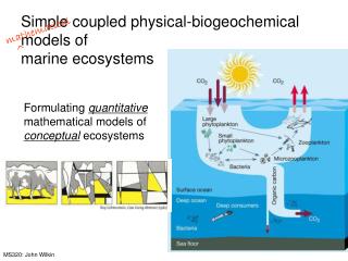
mathematical ^. Simple coupled physical-biogeochemical models of marine ecosystems. Formulating quantitative mathematical models of conceptual ecosystems. MS320: John Wilkin. Why use mathematical models?.

E N D
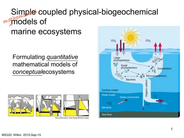
mathematical ^ Simple coupled physical-biogeochemical models of marine ecosystems Formulating quantitative mathematical models of conceptual ecosystems MS320: John Wilkin
Why use mathematical models? • Conceptual models often characterize an ecosystem as a set of “boxes” linked by processes • Processes e.g. photosynthesis, growth, grazing, and mortality link elements of the … • State (“the boxes”) e.g. nutrient concentration, phytoplankton abundance, biomass, dissolved gases, of an ecosystem • In the lab, field, or mesocosm, we can observe some of the complexity of an ecosystem and quantify these processes • With quantitative rules for linking the boxes, we can attempt to simulate the changes over time of the ecosystem state
What can we learn? • Suppose a model can simulate the spring bloom chlorophyll concentration observed by satellite using: observed light, a climatology of winter nutrients, ocean temperature and mixed layer depth … • Then the model rates of uptake of nutrients during the bloom and loss of particulates below the euphotic zone give us quantitative information on net primary production and carbon export – quantities we cannot easily observe directly
Individual plants and animals Many influences from nutrients and trace elements Continuous functions of space and time Varying behavior, choice, chance Unknown or incompletely understood interactions Lump similar individuals into groups express in terms of biomass and C:N ratio Small number of state variables (one or two limiting nutrients) Discrete spatial points and time intervals Average behavior based on ad hoc assumptions Must parameterize unknowns Reality Model
The steps in constructing a model • Identify the scientific problem(e.g. seasonal cycle of nutrients and plankton in mid-latitudes; short-term blooms associated with coastal upwelling events; human-induced eutrophication and water quality; global climate change) • Determine relevant variables and processes that need to be considered • Develop mathematical formulation • Numerical implementation, provide forcing, parameters, etc.
State variables and Processes “NPZD”: model named for and characterized by its state variables State variables are concentrations (in a common “currency”) that depend on space and time Processes link the state variable boxes
Processes • Biological: • Growth • Death • Photosynthesis • Grazing • Bacterial regeneration of nutrients • Physical: • Mixing • Transport (by currents from tides, winds …) • Light • Air-sea interaction (winds, heat fluxes, precipitation)
State variables and Processes Can use Redfield ratio to give e.g. carbon biomass from nitrogen equivalent Carbon-chlorophyll ratio Where is the physics?
Examples of conceptual ecosystems that have been modeled • A model of a food web might be relatively complex • Several nutrients • Different size/species classes of phytoplankton • Different size/species classes of zooplankton • Detritus (multiple size classes) • Predation (predators and their behavior) • Multiple trophic levels • Pigments and bio-optical properties • Photo-adaptation, self-shading • 3 spatial dimensions in the physical environment, diurnal cycle of atmospheric forcing, tides
particulate silicon Silicic acid – important limiting nutrient in N. Pacific gelatinous zooplankton, euphausids, krill copepods ciliates Fig. 1 – Schematic view of the NEMURO lower trophic level ecosystem model. Solid black arrows indicate nitrogen flows and dashed blue arrows indicate silicon. Dotted black arrows represent the exchange or sinking of the materials between the modeled box below the mixed layer depth. Kishi, M., M. Kashiwai, and others, (2007), NEMURO - a lower trophic level model for the North Pacific marine ecosystem, Ecological Modelling, 202(1-2), 12-25.
Soetaert K, Middelburg JJ, Herman PMJ, Buis K. 2000. On the coupling of benthic and pelagic bio-geochemical models. Earth-Sci. Rev. 51:173-201
Phytoplankton concentration absorbs light Att(x,z) = AttSW + AttChl*Chlorophyll(x,z,t) Schematic of ROMS “Bio_Fennel”ecosystem model
Examples of conceptual ecosystems that have been modeled • In simpler models, elements of the state and processes can be combined if time and space scales justify this • e.g. bacterial regeneration can be treated as a flux from zooplankton mortality directly to nutrients • A very simple model might be just: N – P – Z • Nutrients • Phytoplankton • Zooplankton… all expressed in terms of equivalent nitrogen concentration
Mathematical formulation • Mass conservation • Mass M (kilograms) of e.g. carbon or nitrogen in the system • Concentration Cn (kg m-3) of state variable n is mass per unit volume V • Source for one state variable will be a sink for another
Mathematical formulation e.g. inputs of nutrients from rivers or sediments e.g. burial in sediments e.g. nutrient uptake by phytoplankton The key to model building is finding appropriate formulations for transfers, and not omitting important state variables
Some calculus Slope of a continuous function of x is Baron Gottfried Wilhelm von Leibniz 1646-1716
For example:State variables: Nutrient and PhytoplanktonProcess: Photosynthetic production of organic matter Large N Small N Michaelis and Menten (1913) vmax is maximum growth rate (units are time-1) kn is “half-saturation” concentration; at N=kn f(kn)=0.5
Average PP saturates at high PAR PPmax 0.5 PPmax From Heidi’s lectures
State variables: Nutrient and PhytoplanktonProcess: Photosynthetic production of organic matter The nitrogen consumed by the phytoplankton for growth must be lost from the Nutrients state variable
Suppose there are ample nutrients so N is not limiting: then f(N) = 1 • Growth of P will be exponential
Suppose the plankton concentration held constant, and nutrients again are not limiting: f(N) = 1 • N will decrease linearly with time as it is consumed to grow P
Suppose the plankton concentration held constant, but nutrients become limiting: then f(N) = N/kn • N will exponentially decay to zero until it is exhausted
Can the right-hand-side of the P equation be negative? Can the right-hand-side of the N equation be positive? … So we need other processes to complete our model.
Coupling to physical processes Advection-diffusion-equation: physics turbulent mixing Biological dynamics advection C is the concentration of any biological state variable
I0 spring summer fall winter
Simple 1-dimensional vertical model of mixed layer and N-P ecosystem • Windows program and inputs files are at: http://marine.rutgers.edu/dmcs/ms320/Phyto1d/ • Run the program called Phyto_1d.exe using the default input files • Sharples, J., Investigating theseasonal vertical structure of phytoplankton in shelf seas, Marine Models Online, vol 1, 1999, 3-38.
I0 spring summer fall winter bloom
I0 spring summer fall winter bloom secondary bloom
I0 spring summer fall winter bloom secondary bloom