Download
1 / 23
230 likes | 501 Views
Methods of Organizing Data. Prepared by: Josefina V. Almeda Professor and College Secretary School of Statistics University of the Philippines, Diliman August 2009. Quantitative Classification of Data * use quantitative classification if the observed values of the

E N D
Methods of Organizing Data Prepared by:Josefina V. AlmedaProfessor and College SecretarySchool of StatisticsUniversity of the Philippines, DilimanAugust 2009
Quantitative Classification of Data * use quantitative classification if the observed values of the data are either a result of count or measurement * organize this type of data in tabular form in the form of a frequency distribution table. Frequency distribution is a summarized table wherein the classes are either distinct values or intervals with a frequency count.
Forms of the Frequency Distribution Single value grouping * is a frequency count of observed values wherein classes are distinct values * range of values is short and with many unique values occurring more than once Grouping by class intervals * is a frequency count of observed values wherein the classes are intervals.
Data for Single Value Grouping Suppose we have data on the number of children of 50 currently married women using any modern contraceptive method. Construct a summary table for the data set below.
Example of Single Value Grouping Distribution of Currently Married Women Using Any Modern Method of Contraceptive by Number of Children: No. of Frequency of Children Married Women % 0 7 14 1 8 16 2 11 22 3 14 28 4 8 16 5 2 4 TOTAL 50 100
Definition of Terms Used in a Frequency Distribution Table Class intervalcontains the numbers defining a class. Class frequencyis the number of observations falling under a class interval. Class limitsare the end numbers of a class interval. * The lower class limit (LCL) is the lower end of the class interval and the upper class limit (UCL) is the upper end of the class interval. * The number of digits of the class limits should be the same as the number of digits of the raw data. Open class interval is a class interval with either no lower class limit or upper class limit.
Class boundaries are the true class limits. * There are no gaps in the class boundaries. * The number of decimal places is one more than the number of decimal place of the class limits. * The lower class boundary (LCB) is average of the lower class limit of the class interval and the upper class limit of the preceding class interval. * The upper class boundary (UCB) is the average of the upper class limit of the class interval and the lower class limit of the next class interval.
Class size is the size of the class interval. * It is the difference between two successive lower class limits, or two successive upper class limits, or two successive lower class boundaries, or two successive upper class boundaries. Class mark is the midpoint of a class interval. * It is the average of the lower class limit and the upper class limit or the average of the lower class boundary and upper class boundary of a class interval. Modal class is the class interval having the highest frequency.
Steps in Constructing a Frequency Distribution Table • Determine an adequate number of classes (K). • * The number of classes should not be too many or not • too few. • * Usually, the number of classes is between 5 and 20. • * The class intervals should be non-overlapping. • 2. Determine the range (R). Range = Maximum – Minimum • 3. Calculate the approximate class size (C’). • C’ = R/K • 4. Determine the class size (C ) by rounding off C’ to a number that is easy to work with. We recommend class sizes of multiples of 5, 10, 15, 20, etc.
List the required number (K) of class intervals. • * Start with the lower class limit of the lowest class • interval. • * Its value should be less or equal to the minimum value of the data set. • * Add the class size (C) to the lower class limit to get • the next lower class limit. • * The last class interval should include the maximum • value. • Tally the frequency for each class interval. • 7. Sum the frequency column and check against the total number of observations.
TABLE 3. Magnitude of Poor Population in the Philippines: 2000
1 Districts of NCR cover the following: 1st District – Manila; end District – Mandaluyong, Marikina, Pasig, Quezon City and San Juan; 3rd District - Valenzuela, Kaloocan City, Malabon and Navotas; and 4th District – Las Pinas, Makati, Muntinlupa, Paranaque, Pasay City, Pateros, and Taguig. 2 Zamboanga Sibugay was part of Zamboanga del Sur in 2000. Thus, 2000 estimates of Zamboanga del Sur includes Zamboanga Sibugay 3 Isabela City was part of Basilan in 2000. Thus, 2000 estimates of Basilan still includes Isabela City. 4 Davao del Norte estimates for 2000 include Compostela Valley. Source: National Statistical Coordination Board
TABLE 4. Sorted Data (Array) of Magnitude of Poor Population for the 82 provinces of the Philippines: 2000
TABLE 5. Frequency Distribution Table on Magnitude of Poor Population for the 82 Provinces of the Philippines: 2000
Example: This illustrates the use of appropriate column labels in a frequency distribution table. TABLE 6. Frequency Distribution Table of the Magnitude of Poor Population in the Phils: 2000
TABLE 7. Frequency Distribution Table with Class Boundaries and Class Marks
Relative Frequency and Relative Frequency Percentage Relative frequency * divide the class frequency of a class interval to the number of observations * the sum of the relative frequency column is one Relative frequency percentage * multiply the relative frequency by 100 * the sum of the relative frequency percentage column is one hundred percent.
TABLE 8. Frequency Distribution Table with Relative Frequency and Relative Frequency Percentage
TABLE 9. Frequency Distribution Table with Less than Cumulative Frequency and Greater than Cumulative Frequency Distributions
Graphical Representation of the Frequency Distribution • Frequency Histogram - use the class frequency on the vertical axis and the class boundaries on the horizontal axis • Frequency Polygon - use the class frequency on the vertical axis and the class mark on the horizontal axis