Download
1 / 40
400 likes | 570 Views
The Demand Side II. Investment. Applied Macro Theory Course. Supervised By: Prof Mohammad Al-Sekka. Presented By: Halal Alshbaili. Agenda. Manufacturing & Investment. Investment In Housing Conclusion Application on Kuwait. Introduction. I. Introduction.

E N D
The Demand Side II. Investment Applied Macro Theory Course. Supervised By: Prof Mohammad Al-Sekka. Presented By: Halal Alshbaili.
Agenda. • Manufacturing & Investment • Investment In Housing • Conclusion • Application on Kuwait. Introduction
I. Introduction. Investment Expenditure includes spending on a large variety of assets. Investment can be further broken in two:
I. Introduction.1. Fixed Investment . Fixed Investment is gross fixed investment , or gross domestic fixed capital formation.
I.1ntorduction.I. Fixed Investment What is the interest in studying investment? Capital stock is the main reason. In order to calculate it, it is not enough to have the level of gross investment , we need also to know how much capital is being lost. There are two ways to measure this:
I. Introduction.1. Fixed Investment Gross Capital Stock : Includes the value of all capital goods that have not been scrapped. GK(t) = GK(t-1) + GI(t) – S(t) GK(t)= the gross capital stock at the end of period (t) GI(t)= gross investment during period (t) S(t)= scrapping in period (t) Net Capital Stock : Includes the value of all capital goods net of depreciation. NK(t) = NK(t-1) + GI(t) – D(t) NK(t)=net capital stock at the end of period (t) D (t) = Depreciation
1. Introduction.1.1 Fixed Investment. Which measure of capital should we use? Finance Productive Capacity Gross Capital Stock Net Capital Stock
I. Introduction.1. Fixed Investment. GK(t) = GI(t) – S(t) NK(t) = GI(t) – D(t)
1. Introduction.II. Investment in Stock. It is important to distinguish between changes in the value of stocks that are result of inflation and the physical change in stocks.
1. Introduction.II. Investment in Stock. • The demand of stocks is clearly related to current level of output.
II. Manufacturing Investment.1. Investment and Output. • The Theory that can be used to explain the case of manufacturing investment is the Flexible Accelerator. • The Assumptions: 1) The Capital stock adjustment mechanism: Desired capital stock Actual capital stock Fraction 2) The Capital–Output ratio ( ) *Putting These two equations together:
II. Manufacturing Investment.1. Investment and Output. • The version that is used is the following : • - By Estimating this equation we get the following : • If we assume that firms have a desired ratio of stocks to output, The Flexible Accelerator, could be applied to stock building, we finally get:
II. Manufacturing Investment.1. Investment and Output. • To see how well these equations variations investment in manufacturing consider the following figure:
II. Manufacturing Investment.II. Investment and Profitability. • Investment should be dependent on profitability for two reasons : • Firms are assumed to maximize profits. • High profits provides an incentive to invest which is dependent on two factors: The profits the firms expect to obtain on new investment. The cost of obtaining finance. Tobin’s ‘q’
II. Manufacturing Investment.II. Investment and Profitability. • Estimated the cost of capital ,the rate of return on capital, and the value of q that result from them are shown at the following:
II. Manufacturing Investment.III. Profits & the availability of finance • Another method of linking profits to investment is by arguing that high profits provide the funds that firms need to finance investment. • How can this argument make sense? Only when the capital market becomes imperfect * Imperfections can be raised in a number of ways: 1) Borrowing and Lending rates may be differ 2) Transaction costs may be associated with borrowing &lending
II. Manufacturing Investment.III. Profits & the Availability of Finance. • Tobin’s ‘q’ • Can be defined in two ways: 1) The ratio of the rate of return on capital ( R ) to the cost of capital ( ) 2) The ratio of the market value of a firm, V, to the value Of its capital stock at replacement cost .
II. Manufacturing Investment.III. Profits & the availability of finance. • These two definitions are equivalent by : As = • The of cost of capital • It follows that:
II. Manufacturing Investment.III. Profits & the Availability of Finance. The figure clearly shows a correlation between saving and investment.
III. Investment In Housing. • It is apparent that Total Investment is the sum of both the Public and Private investments.
III. Investment In Housing. • Private–sector can explained by the theory that the market price depends on supply and demand for the stock of housing. • The demand : Dependent on several factors such as household incomes and the cost of mortgages. • The supply: Dependent on the prices of housing relative to the cost of building new housing.
III. Investment In Housing. • The figure shows that there is close connection between the real price of housing and investment on housing.
III. Investment In Housing. The figure shows the changes in two variables that make up the real price of housing.
Conclusion. • Investment is highly dependant on expectations, giving it an unpredictable nature. • Because of this, Investment can be very hard to explain. • The Accelerator Model mentioned earlier has the highest success rate, making Investment more predictable.
Application on Kuwait
Investment Chapter: Application on Kuwait. • GI ( Gross Investment)= the total capital Formation. • GI= calculated in Millions Kuwaiti Dinar. • Data calculated from 1971-2007. As you can see that total is fluctuate with raising trend
Investment Chapter: Application on Kuwait. • GDP= gross domestic production . • GDP is taken from constant price on 2000. • The data calculated from 1971-2007. The GDP trend was highly fluctuated pre-Occupation then it rose sharply and Steadily post-Occupation.
Investment Chapter: Application on Kuwait. Ratio= GI/ GDP. From 1971-2007. • The ratio • Is cut as we • can see • due to Iraqi • occupation.
Investment Chapter: Application on Kuwait. • Gross Capital Stock : GK(t) = GK(t-1) + GI(t) – S(t) GK(t)= the gross capital stock at the end of period (t) GI(t)= gross investment during period (t) S(t)= scrapping in period (t Thus we can not apply this formula on the case of Kuwait economy as the data of scrapped is not available. We can apply this formula as all the data necessary is available (more on that later).
Investment Chapter: Application on Kuwait. 2. Net Capital Stock : • NK :gross fixed capital formation which is calculated in million KD , from 1971-2007 . • NK(t) = NK(t-1) + GI(t) – D(t) • NK(t)=net capital stock at the end of period (t) • D (t) = Depreciation NK= 0.112lagNk+0.899GI+(-0.09Dep)
Investment Chapter: Application on Kuwait. Although there are two variables (lagnk & Dep) are insignificant The R -square is very high (99%) which allowed the fitted line to be so close to the actual one, this is obvious can on the figure below.
Investment Chapter: Application on Kuwait. Using the case of manufacturing investment to explain how the level of aggregate output is clearly affecting firms investment decisions, this can be done by a flexible accelerator =change in gross capital formation starting from 1971to 2007. = is the degree of responsive = is the capital – output ratio. Y = is the GDP at constant price on 2000. = is the actual gross capital formation starting from 1971-2007.
Investment Chapter: Application on Kuwait. • Only one variable is • significant which is • Actual gross investment • at 5% level of test. • R-square and • Adjusted R-square are • very low as we can • notice from the output. • Durbin-Watson test • shows that there is • positive autocorrelation. The following is the result of a flexible accelerator. • From the results shown above , we can obtain the following: • = 0.199 • =6.38
Investment Chapter: Application on Kuwait. • The figure below shown there is highly gap between the actual and the fitted graph this is due to low R-square=0.52 and adjusted R-square=0.50
Investment Chapter: Application on Kuwait. • We can apply the flexible accelerator formula on the case of gross capital formation. • Data from(1971-2007), calculated in million KD =0.26 =4.84
Investment Chapter: Application on Kuwait. • The figure shown below represents the high fluctuation for the actual line than the fitted one, which can be rely on the low R-square and Adjusted R-square(0.51, 0,49 ).
Investment Chapter: Application on Kuwait. • According to the data available for Kuwait The following will be the last equation we can apply to it. = change in capital stock we apply it as change in inventories from 1971-2007 in million KD. = in actual GDP at constant prices in 2000 calculated in million KD = is the lagged capital stock , from 1971-2007 ,calculated in million KD
Investment Chapter: Application on Kuwait. • The output is: • 0.77= represent that for each • 1 KD increase in GDP • The change in capital stock will • Increase by 0.77 • 0.28=represents that for each 1 KD • increase in lagged capital stock • The change in capital stock will • Increase by 0.28 • =0.28 • = 2.75
Investment Chapter: Application on Kuwait. • The figure shown below represents the highly fluctuation for the actual line than the fitted one, which can be rely on the low R-square and Adjusted R-square(0.20, 0,18 ).
Thank you for listening.