Download
1 / 37
370 likes | 482 Views
GAINS & LOSSES BY PRESIDENT’S PARTY IN MIDTERM ELECTIONS. MEAN: VARIANCE: ST. DEV.:. What Does it Mean?. On Average, each observation is 17.7 seats away from the mean seat loss (roughly 18 seats). N(-26, 18)--a normal distribution with a mean of negative 26 and standard deviation of 18

E N D
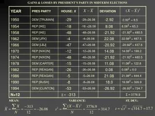
GAINS & LOSSES BY PRESIDENT’S PARTY IN MIDTERM ELECTIONS MEAN:VARIANCE:ST. DEV.:
What Does it Mean? • On Average, each observation is 17.7 seats away from the mean seat loss (roughly 18 seats). • N(-26, 18)--a normal distribution with a mean of negative 26 and standard deviation of 18 • Note: A small SD represents a relatively tight fit of scores around the mean, thereby indicating fewer errors in prediction, whereas a large SD indicates broad dispersion around the mean.
Suppose we were interested in the number of TV ads Senate Candidates run Now You Try • Find the Mean • Compute • Square it: • Add • Divide by N to get the Variance • Take the Square Root of the Variance to get the Standard Deviation *Simulated Data
Mean = -26 St. Dev. = 18 The Seat Loss Example: -80 -62 -44 -26 -8 +10 +28
The 68-95-99.7 Rule This rule tells us that sixty-eight percent of all observations in a normally distributed frequency distribution will be +1 to –1 standard deviations from the mean. The standard deviation in our example is 18. If the distribution of scores (here seat losses) is more or less normally distributed, this means that 68% of the cases are + or – one SD from the mean of 26. So 68% of the cases are between minus 18 seat losses – negative 26 plus minus 18 - 44 (seat losses); negative 26 plus 18 = - 8.
-3sd -2sd -1sd MEAN +1sd +2sd +3sd -80 -62 -44 -26 -8 +10 +28 The 68-95-99.7 rule allows us to predict that in 95% of all midterm election the number of seat losses would be within + 2 sd of the mean -- the mean of 26 minus (18 times 2sd =36 which added to negative 26) equals 62 seats lost. And on the other side 2 standard deviations above the sample mean of -26 is again 36 which adds up to a gain of 10 seats.
Summarizing Variables • It is a good idea to include in a research presentation summary statistics of each of your variables – especially the dependent variable. It is helpful to do this early on in the presentation. • That is, before explaining why something varies, explain how it varies. • Present measures of central tendency and dispersion. • An example or two is also helpful.
For example… • If we are interested in explaining why seat loss varies from one mid-term election to another we would begin with a presentation of its mean and distribution. • “From 1950 to 1994 the president’s party has always lost seats in the House in midterm elections. The average loss has been 26 seats with a standard deviation of 18 seats. The worst seat loss came in 1994 where the Democrats lost 53 seats and the smallest loss of seats was in 1962 when Kennedy’s Democrats lost only 4 seats.” • This should be done for independent variables as they are introduced.
A most important class of frequency distributions is the normal distribution – defined as N [μ, σ] [mu, sigma]. First NDCs describe many natural occurring phenomena, physical, biological, psychological and social. NDCs represent the common case where as people, places and things become more extreme they become less frequent. The average score is most common and the frequency of scores decreases as they diverge from the true score -- the true score being the mean.
All NDCs, not just the ideal bell shape distribution -- is that the area under the curve is the same for all NDCs -- it is100%, meaning that all the cases/observations/people are under the curve. It includes everybody. The frequency distribution contains all the cases or all the people or all scores of the population or sample. • Half the time you are likely fall on one side; the other half of the time the other. • So, if all cases fall under the curve you can see that scores in the middle are more likely to happen than scores at the extreme. The more extreme the score – that is the further the distance to the mean – the less probable is that event occurring just by chance. If you randomly picked people from a NDC, you would expect the mean to be the average size, with few at the extremes. • Because 68% of all cases are + 1 sd of the mean, it means any one individual in the distribution has a .68 probability of having a score within plus or minus 1 sd of the mean.
Mean St. Dev. Notation Population orProbability Sample A standard distribution curve can be defined exactly by its mean and standard deviation
Whatever the mean – as long as the distribution is normally distributed -- and whatever the sd the 68-95-99.7 rule applies -- 68%, two-thirds of all the cases fall within + 1 sd of the mean, 95% of the cases within 2 sd of the mean, and 99.7% of the cases are within + 3 sd of the mean. • The more "peaked" the distribution the smaller the sd, but still, half the cases fall above the mean, half below. • So, sometimes the distance between 1 sd and the mean is wide; there is a lot of variability around the center; whereas at other times the range is narrow. • But what is important here is that although the means of different distributions may differ, as well as the sd of the distributions, IF the distribution is normally distributed -- that is, symmetrical and single peaked -- we can describe the distributions in terms of a “standard normal distribution” , and use the 68-95-99.7 percent rule to talk about thetypicality or extremity of scores -- where exactly a score is located in a NDC.
In the real world many measures tend to bunch up in the middle. The center is the average, with extreme scores less frequent. • It is useful to know how many standard deviations from the mean an observation is. • Call this a z-score.For any individual (i), the Z score tells us how many standard deviations they are from the mean. • We simply take their score (Xi) and subtract the mean, and then divide by the standard deviation. • Doing this allows us to change any value into a standardized value. • Standardized normal distribution has mean of zero and S = 1.
Review of Terms • n = number of people, things or events in a sample • N = number in population • μ = population mean or center of probability distribution • σ = population standard deviation • = sample mean • s = sample standard deviation
where The Standardized Score or Z-score Z is defined for a population as and X is any raw score. But usually, we don’t know the population mean. Σ
Z-Scores • To know how many standard deviations from the sample mean an observation is: Tells us: for any individual (i), how many standard deviations they are from the mean.
We simply take their score (Xi) and subtract the mean, and then divide by the standard deviation. Doing this allows us to change any value into a standardized value. Standardized normal distribution has mean of zero and S = 1. We can create an entire variable that is simply the standardized version of the original variable. Instead of discussing how many seats above or below the mean were lost in an election we can talk about how many standard deviations above or below the mean the seat loss was. This allows us to compare one variable to another on the same scale. We can do this for any interval variable.
Once we have done so, it is easier to make conclusions about the proportion of cases within a given interval. Which is the same as saying the probability of finding the next case in a given interval. The total area under the curve is 1. Half to the right and half to the left. Again, the mean of the standardized normal is zero. We want to know what is the probability of a value between Z=0 and Z=a The area between two points that we want to figure out is our ALPHA-area. We already know some of these values. Between 0 and ∞ .5 0 and -∞ .5
Computing Probabilities from NDC • What is the probability of a score greater than 1 standard deviation above the mean? • + 1 sd: p = .68. • Half of .68: p = .34 • Plus .50 from the other half: • .50 + .34 = .84 • And finally …
From the end of the distribution, compute: 1.00 – .84 = .16 => 16% above 1 sd. Another way : 68% + 1 sd leaves 32% at the tails. Because the NDC is symmetrical , 32/2= 16% above and below at each tail.
From X ~ N with Mean=500 and S=100 what’s the probability of a score between 400 and 600 ? + 1 sd either side of the mean = .68 probability
The interpretation of scores in terms of their relative position helps us interpret their relative probability – the relative extremity or typicality – of some event. Where does a SAT score of 532 stand?? X=532, somewhere between m=500 and +1s, which is at s=600: 500 ——— 532 ——————— 600 m X +1s Score of 532 is somewhere between 500 and 600, but where precisely? What is the exact probability of this event occurring? With the Z score statistic we can interpret the probability of any score occurring anywhere within a normal distribution, say a score of 532, not just whole steps of 1 or 2 or 3 sd steps.
What Does the Z Statistic Accomplish? • Step 1: The population meanцcreates a deviation score: X minus Mean -which converts the distribution mean to zero (themean of a Z distribution is zero); half deviations are above and half below. • Step 2: By dividing deviation by the population sd, the Z score converts the frequency distribution to a standard distribution with a sd equal to 1. So, a Z distribution has a mu of zero and sd of 1, written: N[0, 1]: meaning a normal distribution with a mean of zero and standard deviation of 1. The Z distribution describes all NDCs in units of distance from the center.
In the Z-Score formula, what is the purpose/significance of dividing the deviation between a score [a case or observation] and its distribution mean / by the sd? Said to "standardize" the distribution. Turns every normal distribution in the family of NDC into a standard shape with the same proportion of cases being within 1, 2, 3 or more standard deviations from the mean. IQ test scores are normally distributed with a m = 100 and sd=10. What is the Z-scores for an IQ score of … … 110? Z = (110-100)/10 = 10/10 = Z = 1.0 … 120? (120-100)/10 = 20/10 = Z = 2.0 … 105? (105-100)/10 = 5/10 = Z = 0.50 … 90? (90-100)/10 =-10/10 = Z = -1.0
IQ is normally distributed with a mean of 100 and sd of 10. How do you interpret a score of 109? Use Z-score = (X-m)/s (109-100)/10=9/10=0.90 What does this Z-score of .90 mean? Does not mean 90 percent of cases below this score BUT rather that this Z score is .90 standard units above the mean, almost one sd above the mean.
Standardized Normal Probability Table or simply Z-Table: Luckily, statisticians have already calculated the probabilities for every unit of sd. The tables -- called standardized normal probability tables or simply z-tables -- appear in every statistical text. The z table gives the probability of getting a specific score from a normalized distribution. The z score tells you how distance in units of standard deviation translates into probabilities.
Z Distribution Table • The z scores column. Note that all the z scores in the Table are positive. Rationale: NDCs are symmetrical; therefore plus and minus z scores are equally distant from the mean. Negative z scores are the mirror image of positive z scores. • Column B is the probability (in percent of cases) of a score from the mean to the Z score. • Column C is the probability of a score from Z to the end of the distribution.
IF x=109 and X ~ N[100,100] Variance = 100, so S=10 109 - 100 Z = ————= 0.9 10 What’s the probability of a score above 0.9???
Look at Column C for a Z score of .9 • Find 18.41 • Interpretation: 18.41% of cases fall at or above this Z score of .90 • In probability terms, chance alone would produce a probability of .1841. Or by chance 18.41% of all cases would be at or above this Z score.
Interpret Column B: 31.59% of cases fall between the mean of this distribution and the Z score of .9. What percent of scores by chance would be below the Z score of +.90?
50% + 31.59 = 81.59 81.59% of all scores are below a Z-score of .90.What percentage of scores would be beyond a Z-score of .90? That is at or above an X-score of 109?
Because the total area under the curve is 1.0, we can subtract the probability of .8159 from one: (1-.8159) = .1841meaning that 18.41% of all scores are at or above X = 109 or Z = .90.
USEFULNESS OF Z-SCORES • Describe scores relative to other scores in a single distribution when we divide the deviation by the standard deviation. • The Z-score helps finding the probability of getting a particular value in any normal distribution. • Can make comparisons across different normal distributions, across different samples of individuals or different groups. • The Z score standardizes all NDCs, makes all NDCs comparable even when the means and standard deviations are different.