Numerical quadrature for high-dimensional integrals
490 likes | 669 Views
Numerical quadrature for high-dimensional integrals. L ászló Szirmay-Kalos. Brick rule. Equally spaced abscissa: uniform grid. 0 1 f (z) d z f ( z m ) D z = 1/ M f ( z m ). 0. 1. D z = 1/ M. 0 1 f (z) d z 1/ M f ( z m ).

Numerical quadrature for high-dimensional integrals
E N D
Presentation Transcript
Numerical quadrature for high-dimensional integrals László Szirmay-Kalos
Brick rule Equally spaced abscissa: uniform grid 01f (z) dz f (zm) D z = 1/M f(zm) 0 1 D z = 1/M 01f (z) dz 1/M f(zm)
Error analysis of the brick rule Error = f/2/M·1/M·M= f/2/M=O(1/M) D f 0 1 01f (z) dz 1/M f(zm)
Trapezoidal rule 01f (z) dz (f (zm)+ f (zm+1 ))/2 D z = 1/M f(zm) w(zm) w(zm) = 1 if 1 < m < M 0 1 1/2 if m = 1 or m = M Error = O(1/M) 01f (z) dz 1/M f(zm)w(zm)
Brick rule in higher dimensions 01 01f (x,y) dxdy 1/n j 01f (x,yj) dx 1/n2i j f (xi,yj) = 1/M f(zm) n points M=n2 [0,1]2f (z) dz 1/M f(zm) zm =(xi,yj)
Error analysis for higher dimensions M = n2 samples 01 01f (x,y) dxdy = 1/n j 01f (x,yj) dx fy /2/n 1/n j 1/n (i f (xi,yj) fx /2/n ) fy /2/n = 1/M f(zm) (fx +fy )/2 · M-0.5
Classical rules in D dimensions • Error:f/2 M- 1/D= O(M -1/D) • Required samples for the same accuracy: O( (f/error)D ) • Exponential core • big gaps between rows and columns
Monte-Carlo integration Trace back the integration to an expected value problem [0,1]Df (z) dz= [0,1]Df (z) 1 dz = [0,1]Df (z) p(z) dz = E[f (z) ] f (z) pdf of f (z) Real line E[f (z) ] variance: D2 [f (z) ] p(z)= 1
Expected value estimation by averages f (z) E[f (z) ] f *=1/M f(zm) E[f *]=E[1/M·f(zm)]= 1/M·E[f(zm)]=E[f (z) ] D2[f *]= D2[1/M ·f(zm)]= 1/M 2 ·D2[f(zm)]= if samples are independent! = 1/M 2·M·D2[f(zm)]=1/M·D2[f(z)]
Distribution of the average M=160 E[f (z) ] pdf of f *=1/M f(zm) M=40 Central limit theorem: normal distribution M=10 Three 9s law: Pr{|f *- E[f *] | < 3D[f *]} > 0.999 Probabilistic error bound (0.999 confidence): |1/M f(zm) - [0,1]Df (z) dz | < 3D[f ]/M
Classical versus Monte-Carlo quadratures • Classical (brick rule): f/2 M-1/D • f :variation of the integrand • D dimension of the domain • Monte-Carlo: 3D[f ]/M • 3D[f ]: standard deviation (square root of the variance) of the integrand • Independent of the dimension of the domain of the integrand!!!
Importance sampling Select samples using non-uniform densities f (z) dz= f (z)/p(z) ·p(z) dz = E[f (z)/p(z)] 1/M f(zm)/p(zm) f (z)/p(z) E[f (z)/p(z)] f *=1/M f(zm)/p(zm)
Optimal probability density • Variance of f (z)/p(z) should be small • Optimal case f (z)/p(z) is constant, variance is zero • p(z)f (z) and p(z) dz = 1 p(z) = f (z) / f (z) dz • Optimal selection is impossible since it needs the integral • Practice: where f is large p is large
Numerical integration 01f (z) dz 1/M f (zi) • Good sample points? z1, z2, ..., zn • Uniform (equidistribution) sequences: assymptotically correct result for any Riemann integrable function
Uniform sequence: necessary requirement • Let f be a brick at the center f f (z) dz = V (A) 1 1/M f (zi) = m (A)/M V(A) m(A) lim m (A)/M = V(A) A 0 1
Discrepancy M points • Difference between the relative number of points and the relative size of the area V m points D*(z1,z2,...,zn) = max | m(A)/M - V(A) |
Uniform sequences lim D(z1,...,zn) =0 • Necessary requirement: to integrate a step function discrepancy should converge to 0 • It is also sufficient = +
Other definition of uniformness • Scalar series: z1,z2,...,zn.. in [0,1] • 1-uniform: P(u < zn < v)=(v-u) 0 1 u v
1-uniform sequences • Regular grid: D = 1/2 M • random series: D loglogM/2M • Multiples of irrational numbers modulo 1 • e.g.: {i2 } • Halton (van der Corput) sequence in base b • D b2/(4(b+1)logb) logM/M if b is even • D (b-1)/(4 logb) logM/M if b is odd
Discrepancy of a random series Theorem of large numbers (theorem of iterated logarithm): 1 ,2 ,…, M are independent r.v. with mean E and variance : Pr( limsup | i/M - E | 2 loglogM/M ) = 1 x is uniformly distributed: i (x)= 1 if i(x) < A and 0 otherwise: i/M = m(A)/ M, E = A, 2 = A-A2 < 1/4 Pr( limsup | m(A)/ M - A | loglogM/2M ) = 1
Halton (Van der Corput) seq: Hi is the radical inverse of i i binary form of i radical inverse Hi 0 0 0.0 0 1 1 0.1 0.5 2 10 0.01 0.25 3 11 0.11 0.75 4 100 0.001 0.125 5 101 0.101 0.625 6 110 0.011 0.375 0 4 2 1 3
Uniformness of the Halton sequence i binary form of i radical inverse Hi 0 0 0.000 0 1 1 0.100 0.5 2 10 0.010 0.25 3 11 0.110 0.75 4 100 0.001 0.125 5 101 0.101 0.625 6 110 0.011 0.375 • All fine enough interval decompositions: • each interval will contain a sample before a second sample is placed
Discrepancy of the Halton sequence A4 M bk A1 A2 A3 A |m(A)/M-A| = |m(A1)/M-A1 +…+ m(Ak)/M-Ak | |m(A1)/M-A1|+…+ |m(Ak+1)/M-Ak+1 | k+1 = 1+ logbM D (1+ logM/logb)/ M = O(logM/M) Faure sequence: Halton with digit permutation
Progam: generation of the Halton sequence class Halton { double value, inv_base; Number( long i, int base ) { double f = inv_base = 1.0/base; value = 0.0; while ( i > 0 ) { value += f * (double)(i % base); i /= base; f *= inv_base; } }
Incemental generation of the Halton sequence void Next( ) { double r = 1.0 - value - 0.0000000001; if (inv_base < r) value += inv_base; else { double h = inv_base, hh; do { hh = h; h *= inv_base; } while ( h >= r ); value += hh + h - 1.0; }
2,3,…-uniform sequences • 2-uniform: P(u1 < zn < v1, u2 < zn+1 < v2) = (v1-u1) (v2-u2) (zn ,zn+1 )
-uniform sequences • Random series of independent samples • P(u1<zn< v1, u2< zn+1< v2) = P(u1<zn< v1)P( u2< zn+1< v2) • Franklin theorem: with probability 1: • fractional part of n -uniform • is a transcendent number (e.g. )
Sample points for integral quadrature • 1D integral: 1-uniform sequence • 2D integral: • 2-uniform sequence • 2 independent 1-uniform sequences • d-D integral • d-uniform sequence • d independent 1-uniform sequences
Independence of 1-uniform sequences: p1, p2 are relative primes p2m rows: samples uniform with period p2m p1n p2m cells: samples uniform with period SCM(p1n, p2m) SCM= smallest common multiple p1n columns: samples uniform with period p1n
Multidimensional sequences • Regular grid • Halton with prime base numbers • (H2(i), H3(i), H5(i), H7(i), H11(i), …) • Weyl sequence: Pk is the kth prime • (iP1, iP2, iP3, iP4, iP5, …)
Low discrepancy sequences • Definition: • Discrepancy: O(logD M/M ) =O(M-(1-e)) • Examples • M is not known in advance: • Multidimensional Halton sequence: O(logD M/M ) • M is known in advance: • Hammersley sequence: O(logD-1 M/M ) • Optimal? • O(1/M ) is impossible in D > 1 dimensions
O(logD M/M ) =O(M -(1-e)) ? • O(logD M/M ) dominated by c logD M/M • different low-discrepancy sequences have significantly different c • If M is large, thenlogD M < Me • logD M/M < Me /M = M -(1-e) • Cheat!: e = 0.1, D=10, M = 10100 • logD M = 10010 • Me = 1010
Error of the integrand • How uniformly are the sample point distributed? • How intensively the integrand changes
Variation of the function: Vitali f f Vv xi Vv=limsup |f (xi+1 ) - f (xi )| = 01 |df (u)/du | du
Vitali Variation in higher dimensions f Zero if f is constant along 1 axis f Vv=limsup |f (xi+1,yi+1)-f (xi+1, yi)-f (xi, yi +1)+ f (xi, yi)| = |2f (u,v)/ u v | du dv
Hardy-Krause variation VHK f= VVf (x, y) + VVf (x, 1) +VVf (1, y) = |2f (u,v)/ u v | du dv + 01 |df (u ,1)/du | du +01 |df (1 ,v)/dv | dv
Hardy-Krause variation of discontinuous functions f f Variation: Variation: |f (xi+1,yi+1)-f (xi+1, yi)- f (xi, yi +1) + f (xi, yi)|
Koksma-Hlawka inequalityerror( f ) < VHK •D(z1,z2,...,zn) • 1. Express:f (z) from its derivative f(1)-f(z) = z1 f ’(u)du f(z)=f(1)- z1 f ’(u)du f(z) = f(1)- 01 f ’(u) e(u-z) du e(u-z) e(u) u u z
Express 1/M f(zi) 1/M f (zi) = = f(1)- 01 f ’(u) ·1/M e(u-zi) du = = f(1)- 01 f ’(u) ·m(u) /M du
Express01 f(z)dz using partial integration ab’= ab - a’b 01 f (u) ·1 du = f (u) ·u|01 -01 f ’(u) ·u du = = f(1)- 01 f ’(u) ·u du
Express|1/M f(zi) -01f(z)dz| | 1/M f (zi) - 01 f (z)dz| = = |01 f ’(u) ·(m(u)/M - u) du | = 01 |f ’(u) ·(m(u)/M - u)| du = 01 |f ’(u)| du· maxu| (m(u)/M - u)| = = VHK · D(z1,z2,...,zn) upperbound
Importance sampling in quasi-Monte-Carlo integration Integration by variable transformation: z = T(y) f (z) dz = f (T(y)) | dT(y)/dy | dy z T 1/p(y) = |dT(y)/dy| y
Optimal selection Variation of the integrand is 0: f (T(y)) ·| dT(y)/dy | = const f (z) ·| 1/ (dT-1(z)/dz) | = const y = T-1(z) = zf (u) du /const Since y is in [0,1]: T-1(zmax) = f (u) du /const = 1 const = f (u) du z = T(y) = (inverse of zf (u) du/ f (u) du) (y)
Comparing to MC importance sampling • f (z) dz = E[f (z)/p(z)], p(z) f (z) • 1. normalization: p(z) = f (z)/ f (u) du • 2. probability distributions • P(z)= zp(u) du • 3. Generation of uniform random variable r. • 6. Find sample z by transforming rby the inverse probability distribution: • z = P-1(r)
MC versus QMC? • What can we expect from quasi-Monte Carlo quadrature if the integrand is of infinite variation? • Initial behavior of quasi-Monte Carlo • 100, 1000 samples per pixel in computer graphics • They are assymptotically uniform.
QMC for integrands of unbounded variation Length of discontinuity l |Dom|= l / N N Number of samples in discontinuity M = l N N
Decomposition of the integrand integrand finite variation part discontinuity f s d + = f
Error of the quadrature error (f ) error( s) + error(d ) QMC MC VHK•D(z1,z2,...,zn) |Dom| • 3 f / M = 3 f l • N -3/4 In d dimensions: 3 f l • N -(d+1)/2d
Applicability of QMC • QMC is better than MC in lower dimensions • infinite variation • initial behaviour (n > base = d-th prime number)