Download
1 / 12
120 likes | 364 Views
Numerical Approximations of Definite Integrals. Riemann Sums Numerical Approximation of Definite Integrals Formulae for Approximations Properties of Approximations Example. Riemann Sums.

E N D
Numerical Approximations of Definite Integrals Riemann Sums Numerical Approximation of Definite Integrals Formulae for Approximations Properties of Approximations Example
Riemann Sums A Riemann sum for the integral of a function f over the interval [a,b] is obtained by first dividing the interval [a,b] into subintervals and then placing a rectangle, as shown below, over each subinterval. The corresponding Riemann sum is the combined area of the green rectangles. The height of the rectangle over some given subinterval is the value of the function f at some point of the subinterval. This point can be chosen freely. Taking more division points or subintervals in the Riemann sums, the approximation of the area of the domain under the graph of f becomes better. Mika Seppälä: Numerical Integration
1 Riemann sum 2 Measure of the fineness of the decomposition D of the interval [a,b] into subintervals 3 Definition of the definite integral of the function f over the interval [a,b] Definite Integrals Definitions This definition assumes that the limit does not depend on the various choices in the definition of the Riemann sums. This is true if f is continuous on [a,b]. Mika Seppälä: Numerical Integration
Numerical Approximations of Definite Integrals In view of the definition of the definite integral we may approximate its value by choosing the decomposition D to be a decomposition of the interval [a,b] into subintervals of length (b-a)/n for some positive integer n. The points xj can be freely chosen according to any rule from the intervals [xj -1, xj ] = [a + (i -1)(b - a)/n, a + i (b - a)/n ]. In left rule approximations, xj = xj-1. In mid rule approximations,xj = (xj-1+ xj)/2. In right rule approximations,xj = xj. Mika Seppälä: Numerical Integration
1 Left Rule Approximation 2 Right Rule Approximation Mid Rule Approximation 3 Formulae for Approximations Definitions Mika Seppälä: Numerical Integration
Trapezoidal approximations and Simpson’s Formula Depending on the shape of the function in question, the following approximations are often better approximations than the previously defined approximations: Definitions Trapezoidal Approximation: TRAP(n) = (LEFT(n)+RIGHT(n))/2 Simpson’s Approximation: SIMPSON(n)=(2MID(n)+TRAP(n))/3. Mika Seppälä: Numerical Integration
Properties of Approximations Property This property follows directly from the definitions as illustrated in the above pictures. For an increasing positive function every LEFT(n) is the combined area of rectangles included in the area of the domain bounded by the graph of f. Hence we have the first inequality which also holds if the values of f are not always positive. If f is strictly increasing – like in the above picture – then the above inequalities are also strict. If f is decreasing, then the direction of the above inequalities must be changed. Mika Seppälä: Numerical Integration
Properties of Approximations This follows directly from the definitions. Error Estimates If f is decreasing the above inequalities have to be reversed. These estimates show that the approximations can be made as precise as needed simply by increasing the number n of subintervals. Mika Seppälä: Numerical Integration
Properties of Midpoint Approximations A function which is concave up has the property that its graph lies above any tangent line. This observation leads to the following estimate valid for functions that are concave up. Property The approximations MID(n) give the combined area of rectangles like the one in the picture on the right. The area of the blue rectangle is the same as the area of the blue triangle on the right. Since the triangle is included in the area bounded by the graph of f, the first inequality of the above property follows. The second inequality follows from the fact that if the graph of a function is concave up, then the graph lies below a secant line between the points of intersection. Mika Seppälä: Numerical Integration
Example 1/3 Problem The function to be integrated is decreasing in the interval of integration. Hence we have Solution for any n. For n = 10, we get (compute using Maple) The errors of RIGHT(n) or of LEFT(n) estimates are < 0.1729. Mika Seppälä: Numerical Integration
Example 2/3 Problem In this case the Trapezoidal Approximation and Simpson’s Approximation give better estimates. Solution To be able to apply these estimates correctly we first need to figure out the direction of concavity of the graph of the integrand. By looking at the sign of the second derivative we conclude that the graph of the integrand is concave down in the interval [-1,1] and concave up otherwise. Mika Seppälä: Numerical Integration
Example 3/3 Problem Solution Since the graph of the integrand is concave down in the interval [-1,1] and concave up otherwise we have TRAP(n, [1,2]) here means that we apply the trapezoidal method in the interval [1,2]. The other terms have similar meanings. Computing again with Maple for n = 10 we get Mika Seppälä: Numerical Integration