CPU Scheduling
CPU Scheduling. CPU Scheduling. Basic Concepts Scheduling Criteria Scheduling Algorithms. Objectives. To introduce CPU scheduling, which is the basis for multiprogrammed operating systems To describe various CPU-scheduling algorithms


CPU Scheduling
E N D
Presentation Transcript
CPU Scheduling • Basic Concepts • Scheduling Criteria • Scheduling Algorithms
Objectives • To introduce CPU scheduling, which is the basis for multiprogrammed operating systems • To describe various CPU-scheduling algorithms • To discuss evaluation criteria for selecting a CPU-scheduling algorithm for a particular system
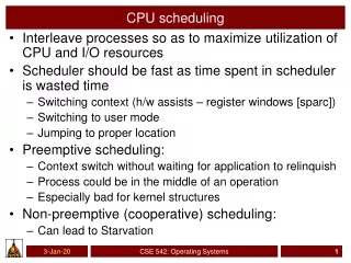
Basic Concepts • Maximum CPU utilization obtained with multiprogramming • CPU–I/O Burst Cycle – Process execution consists of a cycle of CPU execution and I/O wait • CPU burst distribution
CPU Scheduler • Selects from among the processes in ready queue, and allocates the CPU to one of them • Queue may be ordered in various ways • CPU scheduling decisions may take place when a process: 1. Switches from running to waiting state 2. Switches from running to ready state 3. Switches from waiting to ready • Terminates • Scheduling under 1 and 4 is nonpreemptive • All other scheduling is preemptive • Consider access to shared data • Consider preemption while in kernel mode • Consider interrupts occurring during crucial OS activities
Dispatcher • Dispatcher module gives control of the CPU to the process selected by the short-term scheduler; this involves: • switching context • switching to user mode • jumping to the proper location in the user program to restart that program • Dispatch latency – time it takes for the dispatcher to stop one process and start another running
Scheduling Criteria • CPU utilization – keep the CPU as busy as possible • Throughput – # of processes that complete their execution per time unit • Turnaround time – amount of time to execute a particular process • Waiting time – amount of time a process has been waiting in the ready queue • Response time – amount of time it takes from when a request was submitted until the first response is produced, not output (for time-sharing environment)
Scheduling Algorithm Optimization Criteria • Max CPU utilization • Max throughput • Min turnaround time • Min waiting time • Min response time
P1 P2 P3 0 24 27 30 First-Come, First-Served (FCFS) Scheduling ProcessBurst Time P1 24 P2 3 P3 3 • Suppose that the processes arrive in the order: P1 , P2 , P3 The Gantt Chart for the schedule is: • Waiting time for P1 = 0; P2 = 24; P3 = 27 • Average waiting time: (0 + 24 + 27)/3 = 17
P2 P3 P1 0 3 6 30 FCFS Scheduling (Cont.) Suppose that the processes arrive in the order: P2 , P3 , P1 • The Gantt chart for the schedule is: • Waiting time for P1 = 6;P2 = 0; P3 = 3 • Average waiting time: (6 + 0 + 3)/3 = 3 • Much better than previous case • Convoy effect - short process behind long process • Consider one CPU-bound and many I/O-bound processes
Shortest-Job-First (SJF) Scheduling • Associate with each process the length of its next CPU burst • Use these lengths to schedule the process with the shortest time • SJF is optimal – gives minimum average waiting time for a given set of processes • The difficulty is knowing the length of the next CPU request • Could ask the user
P3 P2 P4 P1 3 9 16 24 0 Example of SJF ProcessArriva l TimeBurst Time P10.0 6 P2 2.0 8 P34.0 7 P45.0 3 • SJF scheduling chart • Average waiting time = (3 + 16 + 9 + 0) / 4 = 7
Determining Length of Next CPU Burst • Can only estimate the length – should be similar to the previous one • Then pick process with shortest predicted next CPU burst • Can be done by using the length of previous CPU bursts, using exponential averaging • Commonly, α set to ½ • Preemptive version called shortest-remaining-time-first
Examples of Exponential Averaging • =0 • n+1 = n • Recent history does not count • =1 • n+1 = tn • Only the actual last CPU burst counts • If we expand the formula, we get: n+1 = tn+(1 - ) tn-1+ … +(1 - )j tn-j+ … +(1 - )n +1 0 • Since both and (1 - ) are less than or equal to 1, each successive term has less weight than its predecessor
P1 P3 P4 P2 P1 0 5 1 10 17 26 Example of Shortest-remaining-time-first • Now we add the concepts of varying arrival times and preemption to the analysis ProcessAarriArrival TimeTBurst Time P10 8 P2 1 4 P32 9 P43 5 • Preemptive SJF Gantt Chart • Average waiting time = [(10-1)+(1-1)+(17-2)+5-3)]/4 = 26/4 = 6.5 msec
Priority Scheduling • A priority number (integer) is associated with each process • The CPU is allocated to the process with the highest priority (smallest integer highest priority) • Preemptive • Nonpreemptive • SJF is priority scheduling where priority is the inverse of predicted next CPU burst time • Problem Starvation – low priority processes may never execute • Solution Aging – as time progresses increase the priority of the process
P1 P5 P3 P4 P2 0 6 1 16 18 19 Example of Priority Scheduling ProcessAarriBurst TimeTPriority P1 10 3 P2 1 1 P32 4 P41 5 P5 5 2 • Priority scheduling Gantt Chart • Average waiting time = 8.2 msec
Round Robin (RR) • Each process gets a small unit of CPU time (time quantum q), usually 10-100 milliseconds. After this time has elapsed, the process is preempted and added to the end of the ready queue. • If there are n processes in the ready queue and the time quantum is q, then each process gets 1/n of the CPU time in chunks of at most q time units at once. No process waits more than (n-1)q time units. • Timer interrupts every quantum to schedule next process • Performance • q large FIFO • q small q must be large with respect to context switch, otherwise overhead is too high
P1 P2 P3 P1 P1 P1 P1 P1 0 10 14 18 22 26 30 4 7 Example of RR with Time Quantum = 4 ProcessBurst Time P1 24 P2 3 P3 3 • The Gantt chart is: • Typically, higher average turnaround than SJF, but better response • q should be large compared to context switch time • q usually 10ms to 100ms, context switch < 10 usec
Multilevel Queue • Ready queue is partitioned into separate queues, eg: • foreground (interactive) • background (batch) • Process permanently in a given queue • Each queue has its own scheduling algorithm: • foreground – RR • background – FCFS • Scheduling must be done between the queues: • Fixed priority scheduling; (i.e., serve all from foreground then from background). Possibility of starvation. • Time slice – each queue gets a certain amount of CPU time which it can schedule amongst its processes; i.e., 80% to foreground in RR • 20% to background in FCFS
Multilevel Feedback Queue • A process can move between the various queues; aging can be implemented this way • Multilevel-feedback-queue scheduler defined by the following parameters: • number of queues • scheduling algorithms for each queue • method used to determine when to upgrade a process • method used to determine when to demote a process • method used to determine which queue a process will enter when that process needs service
Example of Multilevel Feedback Queue • Three queues: • Q0 – RR with time quantum 8 milliseconds • Q1 – RR time quantum 16 milliseconds • Q2 – FCFS • Scheduling • A new job enters queue Q0which is servedFCFS • When it gains CPU, job receives 8 milliseconds • If it does not finish in 8 milliseconds, job is moved to queue Q1 • At Q1 job is again served FCFS and receives 16 additional milliseconds • If it still does not complete, it is preempted and moved to queue Q2