Download

1 / 45
450 likes | 533 Views
A robust approach catering to uncertainties & exchange rate variances in the capacitated international sourcing problem. Discusses scenario modeling, supplier selection, & decision-making under risk.

E N D
Adaptive Memory Programming for the Robust Capacitated International Sourcing Problem José Luis González-Velarde Tecnológico de Monterrey, México Rafael Martí Universitat de València, Spain.
The capacitated sourcing problem M Suppliers N Plants Setup Cost Demand Capacity 1 … i … m 1 … j … n d1 di dm f1 fi fm b1 bi bm cij
The International Problem with Scenarios • The variant proposed by González-Velarde and Laguna (2004) • Suppliers and plants are located worldwide, thus exchange rates must be considered in the costs. • Variations of exchange rates in different periods (scenarios) affect the quality of the solution. • The demand of the plants varies in different periods (scenarios)
Planteo del problema • Seleccionar un subconjunto de un conjunto disponible de proveedores potenciales localizados internacionalmente. • El proceso de selección involucra la optimización de una función objetivo la cual puede ser, un costo, o bien una medida de utilidad.
Abastecedores Plantas
Abastecedores: Costo fijo, capacidad
Costo por abastecer
Seleccionar un proveedor implica un costo fijo asociado con actividades tales como transferencia de tecnología, programas de calidad, certificaciones ISO y capacitación de personal. • Satisfacer las demandas de las plantas implica costos variables incluyendo la compra y costos de transporte desde el proveedor hasta la planta
Más aún, el hecho de que varios países estén involucrados en el proceso implica que las tasas de cambio entre las diferentes monedas deben también considerarse al tomar la decisión.
Abastecedores Seleccionados
Variables de control para escenario s1
Variables de control para escenario s2
Suposiciones • La primera se refiere a la capacidad de los proveedores, la cual puede considerarse finita o infinita. Si la capacidad se considera finita, el problema es más difícil. • La suposición más importante tiene que ver con la incertidumbre de los parámetros clave del problema.
Ya que los costos se ven afectados por las condiciones macroeconómicas de los países donde los proveedores y las plantas están situados, una formulación realista debe considerar la incertidumbre asociada con los cambios de estas condiciones.
Optimización Robusta • Un enfoque común es capturar la incertidumbre usando escenarios y formulando un problema determinístico equivalente.
Parámetros de incertidumbre • Consideramos que la demanda es incierta y la modelamos vía escenarios. • Generamos explícitamente escenarios donde la demanda está relacionada con el precio de las partes, el cual a su vez se ve afectado por la tasa de cambio de las monedas involucradas en cada transacción.
Modelo • N : conjunto de plantas internacionales {1,2,...,n} • M : conjunto de proveedores internacionales potenciales {1,2,...,m} • S : conjunto de escenarios
Parámetros • fi: costo fijo del desarrollo del proveedor i • cij : costo total unitario de transporte desde el proveedor i hasta la planta j • bi: capacidad del proveedor i
Parámetros (cont.) • djs : demanda de la planta j en el escenario s • eis : tasa de cambio en el país del proveedor i en el escenario s • ps : probabilidad de que occurra el escenario s
Variables de decisión • Variables de diseño • yi : 1 si el proveedor i se contrata, 0 en otro caso • Variables de control • xijs : embarque del proveedor i a la planta j en el escenario s
Restricciones • Consideramos que para cada escenario s, la demanda en la planta j debe satisfacerse:
Restricciones (cont.) • Consideramos también que para cada escenario s, la capacidad del proveedor i no puede excederse.
Función objetivo • Una función objetivo posible para este problema puede caracterizarse como sigue:
Optimización robusta • No da cuenta adecuadamente del riesgo, haciéndola inapropiada para tomar decisiones cuando hay aversión al riesgo. • Para manejar el riesgo, adoptaremos el enfoque de igualar el riesgo con la variabilidad de los eventos desconocidos.
A first formulation Exchange rates Probability of scenario s Scenarios Select the supplier independently of the scenarios
Penalizing Costs Scenarios Sol. 1 Sol. 2 Sol 1 Sol. 2 1 (0.2) 70 35 47.2 9.6 2 (0.4) 10 20 0 0 3 (0.4) 12 26 0 0.6 E(z) 22.8 25.4 9.44 2.16 Values Deviations
A robust objective function zs is the optimal objective value associated with the transportation problem obtained when the problem above is solved for a particular scenario s. It penalizes only the positive deviations from the expected value (when the objective value in a given scenario exceeds the expected cost)
Solution methodAdaptive Memory Programming • A constructive procedure • Implements frequency-based memory • An improvement method • Selectively applied • No memory structures • A Post-processing • Implements a Path Relinking method
The constructive method • Attractiveness of selecting supplier i:
The constructive method • Penalization to induce diversification:
The constructive method • Each construction starts by creating a list of unassigned suppliers U, (i.e., initially |U| = m). • Then, we restrict this candidate list considering the set U' with the k most attractive suppliers, according to the G’-value. • The next supplier s is randomly selected from the set U', then U is updated (U = U – {s}) and U’ is recalculated. • The method finishes when the sum of the capacities of the selected suppliers is at least as large as D.
The improvement method • The local search procedure examines, for each supplier yi the best alternative supplier for exchange. • The set P of all generated solutions is partitioned into P = A1 U A2 U …U Ak …U An, • Ak consists of all solutions with exactly k suppliers, the local search is only applied to a percentage pr of the best solutions in each set
The improvement method • Consider Sj, the set of generated solutions in which supplier j is selected. • Sj={y e P | yj=1}. • V(j) will measure the relative contribution of supplier j to the quality of the generated solutions. • V(j) is just the average value of the solutions in Sj.
The improvement method • The local search procedure examines, for each supplier yi the best alternative supplier for exchange. • Non selected suppliers yjare then scanned in the order given by the G´´-value. • For each supplier yj we test whether this exchange is feasible in terms of the capacity (we only admit those solutions where the supply exceeds the demand for every scenario). • The first feasible exchange that results in a solution with a lower objective value is performed. The algorithm finishes when no further improvement is possible.
Path Relinking post-processing • For each pair of solutions y′, y′′ in a given Aktwo new solutions are computed • y∩i= min (y′i, y″i) , yUi= max (y′i, y″i) • Then, instead of creating a path between y′ and y″, we create a path between these two new points y∩ and yU. • Let S’ be the set of suppliers selected in y’ but non-selected in y’’. Symmetrically, let S’’ be the set of suppliers non-selected in y’ and selected in y’’.
Computational experiments • We compare with a previous Tabu Search method by Gonzalez-Velarde and Laguna (2004) and with a generic Scatter Search . • We use the set of 90 intances previously reported with 27 scenarios, 10 plants and 10, 15 and 20 suppliers respectively (30 instances each) • Optimal solutions were obtained by complete enumeration (8 hours of run time on average)
Additional 30 larger instances 20 plants and 40 suppliers
Conclusions • We propose a new heuristic based on memory structures for the ROCIS problem • Memory can be as efficient in constructions as in local search methods. • A post-processing marginally improves the results of our solving method.