Capacitated vertex covering
270 likes | 456 Views
Capacitated vertex covering. Guha, Hassin, Khuller, Or. Problem outline A simple 4-approximation via LP-rounding 2-approximation by a primal-dual algorithm 3-Approximation with edge demands Capacitated covering on trees. 資訊四 高孟駿. Vertex covering ﹝ 公車問題 ﹞.

Capacitated vertex covering
E N D
Presentation Transcript
Capacitated vertex covering Guha, Hassin, Khuller, Or • Problem outline • A simple 4-approximation via LP-rounding • 2-approximation by a primal-dual algorithm • 3-Approximation with edge demands • Capacitated covering on trees 資訊四 高孟駿
Vertex covering ﹝公車問題﹞ • Given a graph G = ( V, E ) , a vertex covering of G is a subset A V such that (v1,v2) E , we have either v1 A or v2 A
å w x v v Î v V Vertex covering ﹝公車問題﹞ • Each vertex v is associated with weight wv( That is, we pay cost wv for covering vertex v. ) The problem • Input:a graph G = ( V, E ) and a weight function w:V N0 • Output: a covering function x:V { 0,1 } with minimum NP-complete!!
Capacitated vertex covering • Each vertex v has capacity kv , and may have more than one copy. The problem • Input:a graph G = ( V, E ) with weight function w:V N0 and capacity function k :V N0 • Output: a covering function x:V N0 with minimum cost such that v V , we have # { e | v e E } ≦ xv kv
å å y w x ev v v Î d Î ( ) e v v V Integer programming formulation and simple rounding scheme • We can translate the problem into a linear integer program. • Minimize yeu + yev ≧ 1, e = { u, v } E kvxv – ≧ 0 , v V xv ≧ yev , v e E yev { 0,1 } , v e E xv N0 , v V. Why do we need xv ≧ yev ?
Integer programming formulation • Consider the following complete bipartite graph. • The left hand side has two vertices, each has weight W and capacity p2 . The right hand side has p vertices, each has weight 0 and capacity 1. • The real solution has cost W by setting one left vertex and all right vertices 1, while the fractional takes cost W / p by setting all left vertices 1 / (2p) and all right vertices 1. Bad in rounding!!
é ù 1 å = * * x y ê ú v ev k ê ú Î d ( ) e v v A 4-approximation rounding scheme • Solve the linear program by relaxing the requirement the variables take integral values, i.e. yev ≧ 0 and xv ≧ 0. • We define the rounded value y*ev = 1 if yev ≧ ½ or 0 otherwise. • Define • We claim that this rounding gives a 4-approximation.
å å £ £ * y 2 y 2 k x ev ev v v Î d Î d ( ) ( ) e v e v å * y ev Î d ( ) e v • Let = akv + k’v , 0 ≦ k’v ≦ kv , a ≧ 0 From xv ≧ a / 2 + ( k’v / 2kv ) To show that x*v ≦ 4 xv , it suffices to show that a+1 ≦ 4 [ a / 2 + ( k’v / 2kv ) ] = 2a + 2k’v / kv If a ≧ 1 we are done. If a = 0 , then blahblah….. We’re also done.
å å y w x ev v v Î d Î ( ) e v v V 2-approximation ﹝Different approach﹞ • We’ll give a simple primal-dual algorithm and use the dual solution to bound the approximation ratio. • The primal of the relaxation of original problem Minimize yeu + yev ≧ 1, e = { u, v } E kvxv – ≧ 0 , v V xv ≧ yev , v e E yev ≧ 0 , v e E xv ≧ 0 , v V
å w x v v Î v V å å å a a l ev e e Î d Î Î ( ) e v e e E E The dual linear program • The dual of the relaxation of original problem Maximize kvqv + ≦ wv , v V qv + lev ≧ αe , v e E qv ≧ 0 , v V lev ≧ 0 , v e Eαe ≧ 0 , e E • In particular, we have min = max
Min_Capacitated_Cover for every { u,v } δ’(u) E’ := E’ \ { u,v } δ’(u) := δ’(u) \ { u,v } d’v := d’v – 1if d’v = kvthen Dv := δ’(u)end ifend forend while x*v := |edges assigned to v| / kvreturn x*vend Min_Capacitated_Cover begin E’ := E // unassigned edges V’ := V // closed verticesfor every v V δ’(v) := edges in E’ incident to v d’v := |δ’(v)|if d’v > kv then Dv := {} else Dv := δ’(v)end forwhile E’ ≠ {} choose a vertex u from V’ V’ := V’ \ {u}if d’u > ku then Assign δ’(u) to u else Assign Du to u// for Du \ E’ this is a re-assignmentend if
Algorithm description • At the beginning, all vertices are closed. As the algorithm runs, some vertices may be declared open. • Define a opened vertex v to be low degree if when it is declared open d’(v) ≦ kv , and to be high degree otherwise. • For a low degree vertex u, we assign all edges in Du to it. ( Some edges may be re-assigned in this step, namely, the edges in Du \ E’ ) • For a high degree vertex u, we assign all edges in δ’(u) to it. ( There is no re-assignment in this step. )
Further description , interaction with dual problem • Initially, all the dual variables αe are 0. This is a dual feasible solution. • The dual problem is solved by increasing all the dual variables αe for unassigned edges e E’. • When any of the vertex constraint is met with equality, we mark it open and stop increasing the dual variables of the assigned edges. • To maintain dual feasibility of the edge constraint, we need to increase qv or lev as we increase αe. If the vertex is high degree, then we increase qv. And we increase lev otherwise.
å £ a £ w ( S ) 2 2 w ( opt ) e Î e E Bounding the approximation ratio Theorem Min_Capacitated_Cover returns a 2-approximation for MINIMUM CAPACITATED COVER. proof The algorithm open a multi-set S of vertices. To bound the weight that each vertex ( and all its copies ) contributesto, we charge the weight it produces to the edges assigned to it. We claim that each edge e gets a charge of at most 2αe If this is true, then we have which is the desired bound.
å å = = a w l v ev e Î d Î d ( ) ( ) e v e v Claim We can charge the weight of each open vertex ( and all its copies ) to edges assigned to it such that each edge e gets a charge of at most 2αe . Proof of the claim Consider a low degree vertex v. (i) If d(v) ≦ kv, then Dv = δ(v). We have qv = 0 since we’ll never increase qv in this case. So from two tight constraint We thus can charge the cost of v to all incident edges by charging αe to each e δ(v) (ii) If d(v) > kv and d’(v) = kv at some later time, then |Dv| = kv. We fix qv and subsequently increase lev from then on. For e not in Dv, we have lev = 0.
( ) å å = + = a q l v ev e å å = + = + w k q l k q l Î Î e D e D v v v v v ev v v ev Î d Î ( ) e v e D v So when this vertex is declared open, we have Thus, the cost for the vertex is charged to all edges in Dv . Next consider a high degree vertex v. Let δ’(v) be the set of unassigned edges incident to v when v is declared open. ( Only the edges in δ’(v) can be charged by v . ) Let Rv be the subset of δ’(v) that is re-assigned some later time.In this case we have lev = 0 and αe = qv for all unassigned edge e when the vertex is declared open.
So we have wv = kvqv = kvαe e δ’(v) The cost for a copy of v needs to be charged to kv edges. Write δ’(v) = pvkv + kv’ , where 0 ≦ kv’ < kv. (i) If |Rv| ≧ kv’ then at most pv copies are need. And we can charge all the weight to any of these edges. (ii) If |Rv| < kv’ then we need pv + 1 copies and (pv+1)kv edges to be charged. We first charge all the edges in δ’(v) once and kv - kv’ edges that is not in Rv one more time. From the discussion above, each edge gets charge αe at most twice and the claim is proved.
å å y d w x ev e v v Î d e ( v ) Î v V Approximation with edge demands • In this case, the primal and dual programs become Minimize yeu + yev ≧ 1, e = { u, v } E kvxv – ≧ 0 , v V xv ≧ yev , v e E yev ≧ 0 , v e E xv ≧ 0 , v V
å å a l ev e Î d Î ( ) e v e E Approximation with edge demands • The dual problem Maximize kvqv + ≦ wv , v V qvde + lev ≧ αe , v e E qv ≧ 0 , v V lev ≧ 0 , v e Eαe ≧ 0 , e E
å £ d rk e v Î d ' ( ) e v å > d k e v Î d ' ( ) e v Approximation strategy • We grow αe in proportion to de. If we raise qv , otherwise we raise lev . • We do not perform any re-assignments. • We claim that this gives a 3-approximation. To see, let r be the minimum integer such that
1 å ³ ³ rk d rk v e v 2 Î d ' ( ) e v a = d q e e v å å a = ³ = 2 ( 2 d q ) rk q rw e e v v v v Î d Î d e ' ( v ) e ' ( v ) Approximation strategy (2) • If r > 1 , then we have In this case and we can charge all edges (assigned to v) at most 2αe since • If r = 1 ,
Capacitated covers on trees • We consider the special case that G = ( V, E ) is a tree. • We also consider two variations whether or not the demand can be split so that de = dev + deu. For both case CVCT is NP-hard. Theorem CVCT is NP-hard even when kv = k for all v V. This claim holds in both cases when edge demands can and cannot be split.
å c v Î v S Ì S { 1 , 2 ,..., n } å £ a B v Î v S Theorem CVCT is NP-hard even when kv = k for all v V. This claim holds in both cases when edge demands can and cannot be split. Sketch of the proof We do a reduction from the Knapsack Problem﹝背包問題﹞,which is known to be NP-hard. The Knapsack problem:max ,
0 1 2 3 n n+1 n å > > w w w + n 1 0 v = v 1 Consider the following graph kv = B + 1 for all v = 0,1,…,n+1 wv = cv for v = 1,2,…,n d0,v = av for v = 1,2,…,n d0,n+1 = 1
Capacitated covers on trees • The general case is NP-hard, however, three special cases can be solved in polynomial time. • The first one assumes unit edge demands. Theorem CVCT with unit edge demands can be solved in polynomial time. sketch of the proof
v c1 c2 c3 cn For each vertex v, let Tv be the subtree rooted at v, ev be the edge connecting v and its parent. Let Wvout be the minimum cost of Tv, Wvin be the minimum cost of Tv U {ev} under the restriction that ev is assigned to v. Let Av = the set of children of vFor each u Av , define cu = Wvin – Wvout
Capacitated covers on trees B. The second case assumes unit cost and splitable edge demands. Theorem CVCT with unit vertex cost and splitable edge demands can be solved in polynomial time. sketch of the proof