Download
1 / 49
490 likes | 698 Views
Testing means, part II The paired t-test. Outline of lecture. Options in statistics sometimes there is more than one option One-sample t-test: review testing the sample mean The paired t-test testing the mean difference. A digression: Options in statistics. Example.

E N D
Outline of lecture • Options in statistics • sometimes there is more than one option • One-sample t-test: review • testing the sample mean • The paired t-test • testing the mean difference
Example • A student wants to check the fairness of the loonie • She flips the coin 1,000,000 times, and gets heads 501,823 times. • Is this a fair coin?
Ho: The coin is fair (pheads = 0.5). Ha: The coin is not fair (pheads≠ 0.5). n = 1,000,000 trials x = 501,823 successes Under the null hypothesis, the number of successes should follow a binomial distribution with n=1,000,000 and p=0.5
Binomial test • P = 2*Pr[X≥501,823] P = 2*(Pr[X = 501,823] + Pr[X = 501,824] + Pr[X = 501,825] + Pr[X = 501,826] + ... + Pr[X = 999,999] + Pr[X = 1,000,000]
Central limit theorem The sum or mean of a large number of measurements randomly sampled from any population is approximately normally distributed
Example • A student wants to check the fairness of the loonie • She flips the coin 1,000,000 times, and gets heads 501,823 times. • Is this a fair coin?
Normal approximation • Under the null hypothesis, data are approximately normally distributed • Mean: np = 1,000,000 * 0.5 = 500,000 • Standard deviation: • s = 500
Normal distributions • Any normal distribution can be converted to a standard normal distribution, by Z-score
From standard normal table: P = 0.0001
Conclusion • P = 0.0001, so we reject the null hypothesis • This is much easier than the binomial test • Can use as long as p is not close to 0 or 1 and n is large
Example • A student wants to check the fairness of the loonie • She flips the coin 1,000,000 times, and gets heads 500,823 times. • Is this a fair coin?
A Third Option! • Chi-squared goodness of fit test • Null expectation: equal number of successes and failures • Compare to chi-squared distribution with 1 d.f.
Test statistic: 13.3 Critical value: 3.84
Coin toss example Chi-squared goodness of fit test Normal approximation Binomial test Most accurate Hard to calculate Assumes: Random sample Approximate Easier to calculate Assumes: Random sample Large n p far from 0, 1 Approximate Easier to calculate Assumes: Random sample No expected <1 Not more than 20% less than 5
Coin toss example Chi-squared goodness of fit test Normal approximation Binomial test in this case, n very large (1,000,000) all P < 0.05, reject null hypothesis
Normal distributions • Any normal distribution can be converted to a standard normal distribution, by Z-score
t distribution • We carry out a similar transformation on the sample mean mean under Ho estimated standard error
How do we use this? • t has a Student's t distribution • Find confidence limits for the mean • Carry out one-sample t-test
t has a Student’s t distribution* Uncertainty makes the null distribution FATTER * Under the null hypothesis
Confidence interval for a mean (2) = 2-tailed significance level df = degrees of freedom, n-1 SEY = standard error of the mean
Confidence interval for a mean 95 % Confidence interval: Use α(2) = 0.05
Confidence interval for a mean c % Confidence interval: Use α(2) = 1-c/100
One-sample t-test Null hypothesis The population mean is equal to o Sample Null distribution t with n-1 df Test statistic compare How unusual is this test statistic? P > 0.05 P < 0.05 Reject Ho Fail to reject Ho
The following are equivalent: • Test statistic > critical value • P < alpha • Reject the null hypothesis • Statistically significant
Quick reference summary: One-sample t-test • What is it for? Compares the mean of a numerical variable to a hypothesized value, μo • What does it assume? Individuals are randomly sampled from a population that is normally distributed • Test statistic: t • Distribution under Ho: t-distribution with n-1 degrees of freedom • Formulae:Y = sample mean, s = sample standard deviation
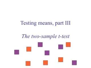
Comparing means • Goal: to compare the mean of a numerical variable for different groups. • Tests one categorical vs. one numerical variable Example: gender (M, F) vs. height
Paired designs • Data from the two groups are paired • There is a one-to-one correspondence between the individuals in the two groups
More on pairs • Each member of the pair shares much in common with the other, except for the tested categorical variable • Example: identical twins raised in different environments • Can use the same individual at different points in time • Example: before, after medical treatment
Paired design: Examples • Same river, upstream and downstream of a power plant • Tattoos on both arms: how to get them off? Compare lasers to dermabrasion
Paired comparisons - setup • We have many pairs • In each pair, there is one member that has one treatment and another who has another treatment • “Treatment” can mean “group”
Paired comparisons • To compare two groups, we use the mean of the difference between the two members of each pair
Example: National No Smoking Day • Data compares injuries at work on National No Smoking Day (in Britain) to the same day the week before • Each data point is a year
Paired t test • Compares the mean of the differences to a value given in the null hypothesis • For each pair, calculate the difference. • The paired t-test is a one-sample t-test on the differences.
Hypotheses Ho: Work related injuries do not change during No Smoking Days (μ=0) Ha: Work related injuries change during No Smoking Days (μ≠0)
Caution! • The number of data points in a paired t test is the number of pairs. -- Not the number of individuals • Degrees of freedom = Number of pairs - 1 Here, df = 10-1 = 9
Critical value of t Test statistic: t = 2.45 So we can reject the null hypothesis: Stopping smoking increases job-related accidents in the short term.
Assumptions of paired t test • Pairs are chosen at random • The differences have a normal distribution It does not assume that the individual values are normally distributed, only the differences.
Quick reference summary: Paired t-test • What is it for? To test whether the mean difference in a population equals a null hypothesized value, μdo • What does it assume? Pairs are randomly sampled from a population. The differences are normally distributed • Test statistic: t • Distribution under Ho: t-distribution with n-1 degrees of freedom, where n is the number of pairs • Formula: