Testing means, part III The two-sample t-test

1. Testing means, part IIIThe two-sample t-test

2. One-sample t-test Null hypothesis The population mean is equal to o Sample Null distribution t with n-1 df Test statistic compare How unusual is this test statistic? P > 0.05 P < 0.05 Reject Ho Fail to reject Ho

3. Paired t-test Null hypothesis The mean difference is equal to o Sample Null distribution t with n-1 df *n is the number of pairs Test statistic compare How unusual is this test statistic? P > 0.05 P < 0.05 Reject Ho Fail to reject Ho

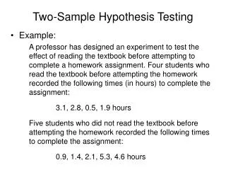
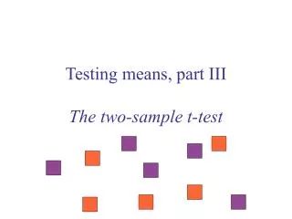
4. Comparing means • Tests with one categorical and one numerical variable • Goal: to compare the mean of a numerical variable for different groups.

5. Paired vs. 2 sample comparisons

6. 2 Sample Design • Each of the two samples is a random sample from its population

7. 2 Sample Design • Each of the two samples is a random sample from its population • The data cannot be paired

8. 2 Sample Design - assumptions • Each of the two samples is a random sample • In each population, the numerical variable being studied is normally distributed • The standard deviation of the numerical variable in the first population is equal to the standard deviation in the second population

9. Estimation: Difference between two means Normal distribution Standard deviation s1=s2=s Since both Y1 and Y2 are normally distributed, their difference will also follow a normal distribution

10. Estimation: Difference between two means Confidence interval:

11. Standard error of difference in means = pooled sample variance = size of sample 1 = size of sample 2

12. Standard error of difference in means Pooled variance:

13. Standard error of difference in means Pooled variance: df1 = degrees of freedom for sample 1 = n1 -1 df2 = degrees of freedom for sample 2 = n2-1 s12 = sample variance of sample 1 s22 = sample variance of sample 2

14. Estimation: Difference between two means Confidence interval:

15. Estimation: Difference between two means Confidence interval: df = df1 + df2 = n1+n2-2

16. Costs of resistance to disease 2 genotypes of lettuce: Susceptible and Resistant Do these differ in fitness in the absence of disease?

17. Data, summarized Both distributions are approximately normal.

18. Calculating the standard error df1 =15 -1=14; df2 = 16-1=15

19. Calculating the standard error df1 =15 -1=14; df2 = 16-1=15

20. Calculating the standard error df1 =15 -1=14; df2 = 16-1=15

21. Finding t df = df1 + df2= n1+n2-2 = 15+16-2 =29

22. Finding t df = df1 + df2= n1+n2-2 = 15+16-2 =29

23. The 95% confidence interval of the difference in the means

24. Testing hypotheses about the difference in two means 2-sample t-test

25. 2-sample t-test Test statistic:

26. Hypotheses

27. Null distribution df = df1 + df2 = n1+n2-2

28. Calculating t

29. Drawing conclusions... Critical value: t0.05(2),29=2.05 t <2.05, so we cannot reject the null hypothesis. These data are not sufficient to say that there is a cost of resistance.

30. Assumptions of two-sample t -tests • Both samples are random samples. • Both populations have normal distributions • The variance of both populations is equal.

31. Two-sample t-test Null hypothesis The two populations have the same mean 12 Sample Null distribution t with n1+n2-2 df Test statistic compare How unusual is this test statistic? P > 0.05 P < 0.05 Reject Ho Fail to reject Ho

32. Quick reference summary: Two-sample t-test • What is it for? Tests whether two groups have the same mean • What does it assume? Both samples are random samples. The numerical variable is normally distributed within both populations. The variance of the distribution is the same in the two populations • Test statistic: t • Distribution under Ho: t-distribution with n1+n2-2 degrees of freedom. • Formulae:

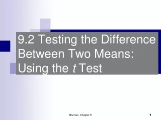
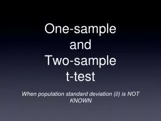
33. Comparing means when variances are not equal Welch’s t test

34. Burrowing owls and dung traps

35. Dung beetles

36. Experimental design • 20 randomly chosen burrowing owl nests • Randomly divided into two groups of 10 nests • One group was given extra dung; the other not • Measured the number of dung beetles on the owls’ diets

37. Number of beetles caught • Dung added: • No dung added:

38. Hypotheses H0: Owls catch the same number of dung beetles with or without extra dung (m1 = m2) HA: Owls do not catch the same number of dung beetles with or without extra dung (m1m2)

39. Welch’s t Round down df to nearest integer

40. Owls and dung beetles

41. Degrees of freedom Which we round down to df= 10

42. Reaching a conclusion t0.05(2), 10= 2.23 t=4.01 > 2.23 So we can reject the null hypothesis with P<0.05. Extra dung near burrowing owl nests increases the number of dung beetles eaten.

43. Quick reference summary: Welch’s approximate t-test • What is it for? Testing the difference between means of two groups when the standard deviations are unequal • What does it assume? Both samples are random samples. The numerical variable is normally distributed within both populations • Test statistic: t • Distribution under Ho: t-distribution with adjusted degrees of freedom • Formulae:

44. The wrong way to make a comparison of two groups “Group 1 is significantly different from a constant, but Group 2 is not. Therefore Group 1 and Group 2 are different from each other.”

45. A more extreme case...