Download
1 / 34
340 likes | 449 Views
Comparison of Observed and Theoretical Fe L Emission from CIE Plasmas. Matthew Carpenter UC Berkeley Space Sciences Laboratory. Collaborators. Lawrence Livermore National Lab Electron Beam Ion Trap (EBIT) Team P. Beiersdorfer G. Brown M. F. Gu H. Chen

E N D
Comparison of Observed and Theoretical Fe L Emission from CIE Plasmas Matthew Carpenter UC Berkeley Space Sciences Laboratory Collaborators Lawrence Livermore National Lab Electron Beam Ion Trap (EBIT) Team P. Beiersdorfer G. Brown M. F. Gu H. Chen UC Berkeley Space Sciences Laboratory J. G. Jernigan Matthew Carpenter, UCB SSL 7/11/2007,
Overview • Introduction to the Photon Clean Method (PCM) • An Example : XMM/RGS spectrum of Ab Dor • PCM algorithm internals • Analysis Modes: Phase I and Phase II solutions • Bootstrap Methods of error analysis • Summary Matthew Carpenter, UCB SSL, 7/11/2007
Photon Clean Method: Principles • Analysis uses individual photon events, not binned spectra • Fitting models to data is achieved through weighted random trial-and-error with feedback • Individual photons span parameter and model space, and are taken to be the parameters • Iteration until quantitative convergence based on a Kolmogorov-Smirnov (KS) test • Has analysis modes which allow divergence from strict adherence to model to estimate differences between model and observed data Matthew Carpenter, UCB SSL, 7/11/2007
Photon Clean Method: Event-Mode Data and Model • Both data and model are in form of EventLists (photon lists) • Monte-Carlo methods are used to generate simulated photons Generation parameters for each photon are recorded Each photon is treated as independentparameter Single simulated photon: Matthew Carpenter, UCB SSL, 7/11/2007
PCM analyzes Simulated Detected sim or Esim Observed Data (Event Form) Simulated Data Data representation inside program Target: AB Dor (K1 IV-V), a young active star and XMM/RGS calibration target Matthew Carpenter, UCB SSL, 7/11/2007
PCM analyzes Simulated Detected sim or Esim Target: AB Dor (K1 IV-V), a young active star and XMM/RGS calibration target The Photon Clean Method algorithm analyzes and outputs models as event lists *** All histograms in this talk are for visualization only Matthew Carpenter, UCB SSL, 7/11/2007
PCM analyzes Simulated Detected sim or Esim Target: AB Dor (K1 IV-V), a young active star and XMM/RGS calibration target The Photon Clean Method algorithm analyzes and outputs models as event lists *** All histograms in this talk are for visualization only Matthew Carpenter, UCB SSL, 7/11/2007
Spectral : “Perfect” information • Each photon in a simulated observation has ideal (model) wavelength and the wavelength of detection == “spectral wavelength” from plasma model Matthew Carpenter, UCB SSL, 7/11/2007
Spectral : “Perfect” information • Each photon in a simulated observation has ideal (model) wavelength and the wavelength of detection == “spectral wavelength” from plasma model • A histogram of the simulated photons’ spectral wavelengths produces sharp lines counts Matthew Carpenter, UCB SSL, 7/11/2007
Adding detector response • Photons are stochastically assigned a “detected wavelength” == “simulated wavelength,” includes redshift, detector and thermal broadening counts Matthew Carpenter, UCB SSL, 7/11/2007
Distribution of Model Parameters • Each photon has individual parameter values which may be taken as elements of the parameter distribution Matthew Carpenter, UCB SSL, 7/11/2007
Distribution of Model Parameters • Each photon has individual parameter values which may be taken as elements of the parameter distribution • The temperature profile of AB Dor is complex; previous fits used 3-temperature or EMD models AB Dor Emission Measure Distribution Histogram of PCM solution counts Three vertical dashed lines are 3-T XSPEC fit from Sanz-Forcada, Maggio and Micela (2003) Matthew Carpenter, UCB SSL, 7/11/2007
PCM Algorithm Progression • Start: Generate initial model + simulated detected photons from input parameter distribution Matthew Carpenter, UCB SSL, 7/11/2007
PCM Algorithm Progression • Start: Generate initial model + simulated detected photons from input parameter distribution Matthew Carpenter, UCB SSL, 7/11/2007
Photon Generator Start: Model Parameter (T) • For CIE Plasma: • Given a temperature (T), AtomDB generates spectral energy (E). • Apply ARF test to determine whether photon is detected • If photon is detected, apply RMF to determine detected energy (E') Result: (T,E,E') + Ancillary Info Matthew Carpenter, UCB SSL, 7/11/2007
PCM Algorithm: Iterate with Feedback Model Esim Iteration: • Generate 1 detected photon Matthew Carpenter, UCB SSL, 7/11/2007
PCM Algorithm: Iterate with Feedback Model Esim Iteration: • Generate 1 detected photon • Replace 1 random photon from model with new photon (E,E',T) Matthew Carpenter, UCB SSL, 7/11/2007
PCM Algorithm: Iterate with Feedback Model Esim Iteration: • Generate 1 detected photon • Replace 1 random photon from model with new photon (E,E',T) • Compute KS probability statistic Feedback Test: If KS probability improves with new photon, keep it; Otherwise, throw new photon away and keep old photon Matthew Carpenter, UCB SSL, 7/11/2007
PCM Analysis Modes Phase I: Constrained Convergence “Re-constrain the Model” • Generates a solution which is consistent with a physically realizable model Matthew Carpenter, UCB SSL, 7/11/2007
PCM Analysis Modes • Phase II: Un-Constrained Convergence: • Iterate until KS probability reaches cutoff value, with Monte-Carlo Markov Chain weighting • Photon distribution is not constrained to model probabilities • Allows individual spectral features to be modified to produce best-fit solution counts Matthew Carpenter, UCB SSL, 7/11/2007
PCM Analysis Modes • Phase II: Un-Constrained Convergence: • Iterate until KS probability reaches cutoff value, with Monte-Carlo Markov Chain weighting • Photon distribution is not constrained to model probabilities • Allows individual spectral features to be modified to produce best-fit solution counts Matthew Carpenter, UCB SSL, 7/11/2007
Determining Variation in Many-Parameter Models • Low-dimensionality models with few degrees of freedom may be quantified using Chi-square test which has a well-defined error methodology. PCM is appropriate for models of high dimensionality where every photon is a free parameter. • For error determination we use distribution-driven re-sampling methods • BootstrapMethod PCM solution counts XPSEC solution Matthew Carpenter, UCB SSL, 7/11/2007
Bootstrap Re-Sampling • Method: • 1) Randomly resample input data set withsubstitution to create new data set • 2) Perform analysis on new data set to produce new outcome • 3) Repeat for n >> 1 re-sampled data sets Matthew Carpenter, UCB SSL, 7/11/2007
Bootstrap Re-Sampling • Method: • 1) Randomly resample input data set withsubstitution to create new data set • 2) Perform analysis on new data set to produce new outcome • 3) Repeat for n >> 1 re-sampled data sets 15.020 14.961 7.622 17.711 21.549 16.062 14.376 13.298 12.833 17.801 Matthew Carpenter, UCB SSL, 7/11/2007
Bootstrap Re-Sampling • Method: • 1) Randomly resample input data set withsubstitution to create new data set • 2) Perform analysis on new data set to produce new outcome • 3) Repeat for n >> 1 re-sampled data sets 15.020 14.961 7.622 17.711 21.549 16.062 14.376 13.298 12.833 17.801 Matthew Carpenter, UCB SSL, 7/11/2007
Bootstrap Re-Sampling • Method: • 1) Randomly resample input data set withsubstitution to create new data set • 2) Perform analysis on new data set to produce new outcome • 3) Repeat for n >> 1 re-sampled data sets 15.020 14.961 7.622 17.711 21.549 16.062 14.376 13.298 12.833 17.801 15.020 7.622 7.622 17.711 21.549 16.062 14.376 14.376 14.376 17.801 Matthew Carpenter, UCB SSL, 7/11/2007
Bootstrap Results AB Dor Emission Measure Distribution Matthew Carpenter, UCB SSL, 7/11/2007
Bootstrap Results AB Dor Emission Measure Distribution Matthew Carpenter, UCB SSL, 7/11/2007
Bootstrap Results AB Dor Emission Measure Distribution Matthew Carpenter, UCB SSL, 7/11/2007
Bootstrap Results AB Dor Emission Measure Distribution Matthew Carpenter, UCB SSL, 7/11/2007
Bootstrap Results AB Dor Emission Measure Distribution Matthew Carpenter, UCB SSL, 7/11/2007
Interpreting the Bootstrap AB Dor Emission Measure Distribution • The variations in the bootstrap solutions estimate errors • The Arithmetic mean of all distributions is plotted as solid line Matthew Carpenter, UCB SSL, 7/11/2007
Interpreting the Bootstrap AB Dor Emission Measure Distribution • The variations in the bootstrap solutions estimate errors • The Arithmetic mean of all distributions is plotted as solid line • Confidence levels are computed along vertical axis of distribution 90% confidence 68% confidence Mean Matthew Carpenter, UCB SSL, 7/11/2007
Summary • The Photon Clean Method allows for complicated parameter distributions • Phase I solution gives best-fit solution from existing models • Phase II solution modifies model to quantify amount of departure from physical models • Bootstrap re-sampling may determine variability of trivial and non-trivial solutions without assumptions about the underlying distribution of the data • As a test of the PCM’s ability to simultaneously model Fe K and Fe L shell line emission, we are using it to model spectra produced by the LLNL EBIT’s Maxwellian plasma simulator mode. Thank You Matthew Carpenter, UCB SSL, 7/11/2007


![Near Infrared Emission Lines From Planetary Nebulae: Lines from H 2 and [Fe III]](https://cdn3.slideserve.com/6332708/near-infrared-emission-lines-from-planetary-nebulae-lines-from-h-2-and-fe-iii-dt.jpg)