Stochastic Network Interdiction: Modeling and Optimization
Explore a two-stage stochastic integer program to minimize expected maximum flow in uncertain interdiction settings. Learn model formulation, decomposition approach, and computational results in interdicting networks.

Stochastic Network Interdiction: Modeling and Optimization
E N D
Presentation Transcript
Stochastic Network Interdiction Udom Janjarassuk
Outline • Introduction • Model Formulation • Dual of the maximum flow problem • Linearize the nonlinear expression • Sample Average Approximation • Decomposition Approach • Computational Results • Further Work
Introduction • Network Interdiction Problem
Introduction (cont.) • Stochastic Network Interdiction Problem (SNIP) • Uncertain successful interdiction • Uncertain arc capacities • Goal: minimize the expected maximum flow • This is a two-stages stochastic integer program • Stage 1: decide which arcs to be interdicted • Stage 2: maximize the expected network flow • Applications • Interdiction of terrorist network • Illegal drugs • Military
Formulation • Directed graph G=(N,A) • Source node rN, Sink node tN • S = Set of finite number of scenarios • ps = Probability of each scenario • K = budget • hij = cost of interdicting arc (i,j)A
Formulation (cont.) where fs(x) is the maximum flow from r to t in scenario s
Formulation (cont.) • uij = Capacity of arc (i,j) A • A’ = A {r,t} • ijs = • yijs = flow on arc (i,j) in scenario s
Formulation (cont.) Maximum flow problem for scenario s
Formulation (cont.) The dual of the maximum flow problem for scenario s is Strong Duality, we have
Linearize the nonlinear expression • Linearize xijijs • Let zijs = xijijs xij = 0 zijs = 0 xij = 1 zijs = ijs • Then we have zijs – Mxij <= 0 – ijs+ zijs <= 0 ijs– zijs + Mxij<= M where M is an upper bound for ijs , here M = 1
Sample Average Approximation • Why? • Impossible to formulate as deterministic equivalent with all scenarios • Total number of scenarios = 2m, m = # of interdictable arcs • Sample Average Approximations • Generate N samples • Approximate f(x) by
Sample Average Approximation(cont.) • Lower bound on f(x)=v* • Confidence Interval
Sample Average Approximation(cont.) • The (1-)-confidence interval for lower bound Where P(N(0,1) z)=1-
Sample Average Approximation(cont.) • Upper bound on f(x) • Estimate of an upper bound (For a fixed x) • Generate T independent batches of samples of size N • Approximate by
Sample Average Approximation(cont.) • Confidence Interval • The (1-)-confidence interval for upper bound Where P(N(0,1) z)=1-
Decomposition Approach • Recall our problem in two-stages stochastic form
Decomposition Approach (cont.) • E[Q(x, s)] is piecewise linear, and convex • The problem has complete recourse – feasible set of the second-stage problem is nonempty • The solution set is nonempty • Integer variables only in first stage • Therefore, the problem can be solve by decomposition approach (L-Shaped method)
Computational results SNIP 4x9 example: Note: 1. Only arcs with capacity in ( ) are interdictable 2. The successful of interdiction = 75% 3. Total budget K = 6
Computational results (cont.) Note: Optimal objective value in [Cormican,Morton,Wood]=10.9 with error 1%
Computational results (cont.) SNIP 7x5 example:
Computational results (cont.) Note: Optimal objective value in [Cormican,Morton,Wood]=80.4 with error 1%
Further work… • Solving bigger instance on computer grid • Using Decomposition Approach