Download
1 / 117
1.18k likes | 1.2k Views
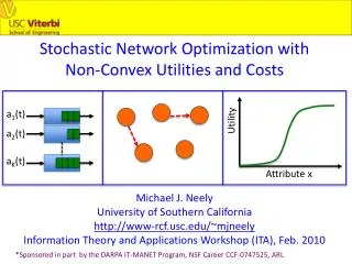
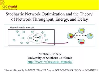
This talk explores the application of stochastic network optimization to general mobile networks, focusing on the energy-delay tradeoff in multi-user wireless downlink systems.

E N D
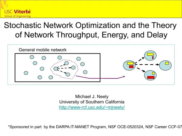
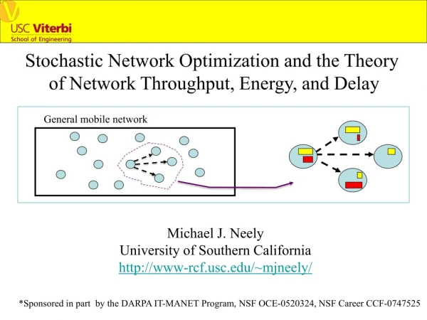
Stochastic Network Optimization and the Theory of Network Throughput, Energy, and Delay General mobile network Michael J. Neely University of Southern California http://www-rcf.usc.edu/~mjneely/ *Sponsored in part by the DARPA IT-MANET Program, NSF OCE-0520324, NSF Career CCF-0747525
Outline: • Analogy between Info Theory and Network Theory • “Capacity” Definitions • Canonical Models • *Overview talk on Stochastic Network Optimization: • History • Landmark Results • Application to general multi-hop stochastic networks • *Focus talk on 1-hop multi-user wireless downlink • Fundamental energy-delay tradeoff • Low complexity achievability • *Details can be found in the following (available on my webpage): • L. Georgiadis, M. J. Neely, L. Tassiulas, “Resource Allocation and Cross-Layer • Control in Wireless Networks,” Foundations & Trends in Networking, vol. 1, • no. 1, pp. 1-144, 2006. • M. J. Neely, “Optimal Energy and Delay Tradeoffs for Multi-User Wireless • Downlinks,” IEEE Transactions on Information Theory, vol. 53, no. 9, pp. 3095-3113, • Sept. 2007.
Part 1: Analogy between info theory and network theory L Capacity Region Λ= Set of all end-to-end rate vectors (or matrices) achievable over a network. l • Information Theory View of Capacity • Optimizes over all maps of symbols into codewords • Results known for point-to-point links • Results known for small 1-hop systems (broadcast/MAC) • Network/Queueing Theory View of Capacity • Sometimes called “transport capacity” [Gupta/Kumar] • Optimizes over all routing/scheduling/resource allocation • Typically “link based” (with some extensions…) • Simplified PHY layer (SINR, Interference Sets, etc.) • Results hold for arbitrarily large networks, with mobility
Part 1: Analogy between info theory and network theory Mathematical Models for a Wireless System (two meaningful perspectives) “info theory” “queueing theory” 1 Wireless Link = AWGN Channel (symbol-by-symbol transmission) 1 Wireless Link = ON/OFF Channel (slot-by-slot packet transmission) Symbols Packet Arrivals + Pr[ON]=p Noise Capacity: Capacity: C = log(1 + SNR) C = p packets/slot Capacity maximizes time avg. bit rate. [Optimizes over all coding strategies.] Capacity = time avg packet transmission rate. [nothing to optimization here] [Basic Queue Stability theory] [very deep math for 1 link]
Part 1: Analogy between info theory and network theory Mathematical Models for a Wireless System (two meaningful perspectives) “info theory” “queueing theory” 1 Wireless Link = AWGN Channel (symbol-by-symbol transmission) 1 Wireless Link = ON/OFF Channel (slot-by-slot packet transmission) Symbols Packet Arrivals + Pr[ON]=p Noise Capacity: Capacity: C = log(1 + SNR) C = p packets/slot Achievability: Random Coding Converse: Sphere-Packet, Fano Achievability: Obvious Converse: Obvious [Basic Queue Stability theory] [very deep math for 1 link]
Part 1: Analogy between info theory and network theory Mathematical Models for a Wireless System (two meaningful perspectives) “info theory” “queueing theory” N-User Gauss. Broadcast Downlink (symbol-by-symbol transmission) N-User Downlink (Fading Channels) (opportunistic packet transmission) l1 ON/OFF bits l2 bits ON/OFF bits lN ON/OFF • Capacity REGION is set of all supportable long term bit rate vectors • Optimizes over all Coding • Strategies • Capacity REGION is set of all • supportable packet arrival rate vectors • Optimizes over all scheduling • strategies • Example: Observe Channel states, • then decide which queue to serve
Part 1: Analogy between info theory and network theory Mathematical Models for a Wireless System (two meaningful perspectives) “info theory” “queueing theory” N-User Gauss. Broadcast Downlink (symbol-by-symbol transmission) N-User Downlink (Fading Channels) (opportunistic packet transmission) l1 ON/OFF bits l2 bits ON/OFF bits lN ON/OFF Capacity Region:all (l1,…, lN) s.t. Capacity Region: all (l1,…, lN) s.t. for all subsets K of users. (degraded Gauss. BC) [Tassiulas & Ephremides ‘93]
p4 p1 p3 p6 p2 p5 Part 1: Analogy between info theory and network theory Mathematical Models for a Wireless System (two meaningful perspectives) “info theory” “queueing theory” N-Node Static Multi-Hop Network (multiple sources and destinations) N-Node Static Multi-Hop Network (multiple sources and destinations) Capacity = Known Exactly(Multi- Commodity Flow Subject to “Graph Family” Link Constraints) Capacity = ??? • Infinite Traffic • Symbol-by-Symbol Transmissions • Interference Channels • Optimize the coding • Pr[Channel k = ON] = pk • Random Packet Arrivals • Optimize Scheduling/Routing
p4 p1 p3 p6 p2 p5 Part 1: Analogy between info theory and network theory Mathematical Models for a Wireless System (two meaningful perspectives) “info theory” “queueing theory” N-Node Static Multi-Hop Network (multiple sources and destinations) N-Node Static Multi-Hop Network (multiple sources and destinations) Capacity = Known Exactly Capacity = ??? • Scheduling Tools: Max Weight • Matching (MWM), Backpressure • Converse Tools: Queue Stability, • Flow Conservation, Optimization • Coding Tools (inner bounds): Net • Coding, Cooperative Trans., etc. • Converse Tools (outer bounds): • cut-sets, multi-terminal info theory
T/R T/R T/R T/R T/R T/R T/R T/R T/R T/R T/R T/R T/R T/R T/R T/R Part 1: Analogy between info theory and network theory Mathematical Models for a Wireless System (two meaningful perspectives) “info theory” “queueing theory” N-Node MANET N-Node MANET Capacity = Known Exactly Scheduling Tools: Max Weight Matching (MWM), Backpressure Routing Converse Tools: Queue Stability, Flow Conservation, Optimization Capacity = ???
T/R T/R T/R T/R T/R T/R T/R T/R T/R T/R T/R T/R T/R T/R T/R T/R Part 1: Analogy between info theory and network theory Mathematical Models for a Wireless System (two meaningful perspectives) “info theory” “queueing theory” N-Node MANET N-Node MANET • Stochastic Network Theory extends to: • Bursty Traffic • Arbitrary Mobility • Performance Optimization • [Neely thesis 2003, Infocom 2005] • [Neely, Modiano, Rohrs JSAC 2005] • [Georgiadis, Neely, Tassiulas F&T 2006] Capacity = ???
Part 2: Overview of Stochastic Network Optimization • What Problems Can be Solved Today? • Slotted time system t = {0, 1, 2, …} • Q(t) = Queue State Vector (possibly multi-hop) • S(t) = “Topology State” (random, chosen by environment) • I(t) = “Control Action” or “Tranmission mode” , I(t) in I • General “Link Transmission Rate Vector Function: • Rate vector(t) = C(I(t), S(t)) • General “Penalty/Reward vector”: • Penalty vector(t) = x(I(t), S(t)) • Queue Evolution: • Q(t) Q(t+1) f() convex hi(x) convex I(t), S(t) Q(t+1) = max[Q(t) – out(t), 0] + in(t)
Part 2: Overview of Stochastic Network Optimization • How is this solved? We have a general and extensive theory: • Lyapunov Drift and Stability for Networks • [Tassiulas & Ephremides TAC 1992, IT 1993] • Drift for Joint Network Stability and Performance Optimization • [Neely thesis 2003, Infocom 2005], [Georgiadis, Neely, Tassiulas F&T 2006] • Virtual Queues • [Neely Infocom 2005, IT 2006], [Georgiadis, Neely, Tassiulas F&T 2006] • Auxiliary Variables and “Flow State” Queues • [Neely, Modiano, Li Infocom 2005], [Georgiadis, Neely, Tassiulas F&T 06] • Alternative Approaches: • Downlink, Linear Utilities [Tsibonis, Georgiadis, Tassiulas Infocom 03] • Flow Based, Static Channels • [Cruz & Santhanam, Infocom 03], [Lin, Shroff CDC 04, Infocom 05] • Fluid Model Analysis for Multi-Hop and General Utilities • [Stolyar, Queueing Systems 05] --- “Primal-Dual” Alg. • Infinite Backlog Assumption, 1-hop downlink [“Prop. Fair” Alg] • [Agrawal, Subramanian, Allerton 02], [Kushner, Whiting Allert. 02] • [Eryilmaz, Srikant Infocom 2005] , [Liu, Chong, Shroff 03]
Part 2: Overview of Stochastic Network Optimization • How is this solved? We have a general and extensive theory: • Lyapunov Drift and Stability for Networks • [Tassiulas & Ephremides TAC 1992, IT 1993] • Drift for Joint Network Stability and Performance Optimization • [Neely thesis 2003, Infocom 2005], [Georgiadis, Neely, Tassiulas F&T 2006] • Virtual Queues • [Neely Infocom 2005, IT 2006], [Georgiadis, Neely, Tassiulas F&T 2006] • Auxiliary Variables and “Flow State” Queues • [Neely, Modiano, Li Infocom 2005], [Georgiadis, Neely, Tassiulas F&T 06] • Note: Our work is unique in that it: • -Solves full problem on the actual queueing network of interest • -Links very nicely to the previous Tassiulas drift framework • -Gets Strongest Results, and Explicit performance-delay Tradeoffs • [O(1/V) ; O(V)] peformance-delay for any network, any utility • Question: Is this the optimal tradeoff?
The Basic Stability Theory for Networks: • Tassiulas & Ephremides [Trans. Autom. Control 1992] • Multi-hop network with Random Packet Arrival Processes • Link Scheduling according to “Feasible Activation Sets” • Lyapunov drift for stability • “Backpressure” Routing and Max-Weight Scheduling • Gives Stability for any rate vector inside capacity region • Does not require knowledge of traffic rates • Tassiulas & Ephremides [Trans. Inform. Theory 1993] • Single-Hop Dynamic Channels • “Opportunistic” scheduling (ie, “channel-aware”) • Lyapunov drift for stability • Max-Weight Algorithm does not require channel statistics or traffic arrival rates, gets stability whenever possible
Quick Description of “Backpressure Routing” and “Max-Weight Scheduling”: n n [Red data is destined for red node, Yellow data is destined for yellow node] • No pre-defined routes! • Optimal Link Activation Set determined by a max-weight rule • “Which packet to send over a link” is determined by a differential • backlog index (backpressure) • The max-weight link activation can be NP hard for networks with • interference, but is trivial (and distributed) for orthogonal links
Quick Description of “Backpressure Routing” and “Max-Weight Scheduling”: n n [Red data is destined for red node, Yellow data is destined for yellow node] • No pre-defined routes! • Optimal Link Activation Set determined by a max-weight rule • “Which packet to send over a link” is determined by a differential • backlog index (backpressure) • The max-weight link activation can be NP hard for networks with • interference, but is trivial (and distributed) for orthogonal links
Quick Description of “Backpressure Routing” and “Max-Weight Scheduling”: n n [Red data is destined for red node, Yellow data is destined for yellow node] • No pre-defined routes! • Optimal Link Activation Set determined by a max-weight rule • “Which packet to send over a link” is determined by a differential • backlog index (backpressure) • The max-weight link activation can be NP hard for networks with • interference, but is trivial (and distributed) for orthogonal links
An Abbreviated History of Lyapunov Drift for Network Stability: • (for various computer networks and switching systems) • Tassiulas & Ephremides (Backpressure, Max-Weight) [1992, 1993] • Kumar & Meyn [1995] • McKeown, Anantharam, Walrand [1996, 1999] • Kahale & Wright [1997] • Andrews, Kumaran, Ramanan, Stolyar, Whiting [2001] • Leonardi, Mellia, Neri, Marsan [2001] • Neely, Modiano, Rohrs [2003, 2005] Extends to MANETs • Performance Optimization (time varying channels) but with • no queueing or stability constraints (infinite backlog assumption): • R. Agrawal, V. Subramanian [2002] (“Proportionally Fair Alg”) • Kushner, Whiting [2002] (“Proportionally Fair Alg”) • Liu, Chong, Shroff [2003]
Corresponding Results for Static Networks (non-stochastic): • These use static convex optimization theory to maximize • network utility. Lagrange multipliers are “shadow prices.” There is either • no queueing analysis, or approximate queueing analysis. • Wireline Networks, Fixed Route Selection, Flow Based • Kelly [1997] • Kelly, Maullou, Tan [1998] • Low, Lapsley [1999] • Wireless Networks, Fixed Route Selection, Flow Based • Xiao, Johansson, Boyd [2001] • Lee, Mazumdar, Shroff [2002] • Julian, Chiang, O’Neill Boyd [2002] • Chiang [2004, 2005] • Scheduling for Utility Optimization (static networks) • Cruz & Santhanam [2003] (scheduling decisions are chosen over time) • Lin & Shroff [2004, 2005] (scheduling decisions are chosen over time)
Work on Utility Optimization for Stochastic Networks: • Wireless Downlink, Time Varying Channels, Infinite Data, No Queueing • R. Agrawal, V. Subramanian [2002] (“Proportionally Fair Alg”) • Kushner, Whiting [2002] (“Proportionally Fair Alg”) • Liu, Chong, Shroff [2003] • Joint Stability and Performance Optimization (Time Varying Channels): • Tsibonis, Georgiadis, Tassiulas [2003] • Solves downlink with special structure, and with linear utilities • Neely [2003, 2005] “Dual Method” • Solves the general problem! (multi-hop, stochastic, concave utilities) • Obtains explicit [O(1/V), O(V)] utility-delay tradeoff! • Stolyar [2005] “Primal-Dual Method” • A different approach to the general problem, solves on a fluid model • Eryilmaz & Srikant [2005] “Dual Method” • Downlink, infinite backlog, fluid model analysis • Lee, Mazumdar, Shroff [2006] • Stochastic gradients, flow based, infinite backlog
S1(t) {ON, OFF} l1 “Proportionally Fair” algorithm (designed for infinite backlog) l2 S2(t) {ON, OFF} λ2 λ2 λ1 λ1 Input Rate Output Rate [Example from Neely, Modiano, Li Infocom 2005, TON 2008]
S1(t) {ON, OFF} l1 “Proportionally Fair” algorithm (designed for infinite backlog) l2 S2(t) {ON, OFF} λ2 λ2 λ1 λ1 Input Rate Output Rate [Example from Neely, Modiano, Li Infocom 2005, TON 2008]
S1(t) {ON, OFF} l1 “Proportionally Fair” algorithm (designed for infinite backlog) l2 S2(t) {ON, OFF} λ2 λ2 λ1 λ1 Input Rate Output Rate [Example from Neely, Modiano, Li Infocom 2005, TON 2008]
S1(t) {ON, OFF} l1 “Proportionally Fair” algorithm (designed for infinite backlog) l2 S2(t) {ON, OFF} λ2 λ2 λ1 λ1 Input Rate Output Rate [Example from Neely, Modiano, Li Infocom 2005, TON 2008]
S1(t) {ON, OFF} l1 “Proportionally Fair” algorithm (designed for infinite backlog) l2 S2(t) {ON, OFF} λ2 λ2 λ1 λ1 Input Rate Output Rate [Example from Neely, Modiano, Li Infocom 2005, TON 2008]
S1(t) {ON, OFF} l1 “Proportionally Fair” algorithm (designed for infinite backlog) l2 S2(t) {ON, OFF} λ2 λ2 λ1 λ1 Input Rate Output Rate [Example from Neely, Modiano, Li Infocom 2005, TON 2008]
S1(t) {ON, OFF} l1 “Proportionally Fair” algorithm (designed for infinite backlog) l2 S2(t) {ON, OFF} λ2 λ2 λ1 λ1 Input Rate Output Rate [Example from Neely, Modiano, Li Infocom 2005, TON 2008]
S1(t) {ON, OFF} l1 “Proportionally Fair” algorithm (designed for infinite backlog) l2 S2(t) {ON, OFF} λ2 λ2 λ1 λ1 Input Rate Output Rate [Example from Neely, Modiano, Li Infocom 2005, TON 2008]
S1(t) {ON, OFF} l1 “Proportionally Fair” algorithm (designed for infinite backlog) l2 S2(t) {ON, OFF} λ2 λ2 λ1 λ1 Input Rate Output Rate [Example from Neely, Modiano, Li Infocom 2005, TON 2008]
S1(t) {ON, OFF} l1 “Proportionally Fair” algorithm (designed for infinite backlog) l2 S2(t) {ON, OFF} λ2 λ2 λ1 λ1 Input Rate Output Rate [Example from Neely, Modiano, Li Infocom 2005, TON 2008]
S1(t) {ON, OFF} l1 “Max-Weight” algorithm (designed only to achieve stability, Tass. & Eph. 93) l2 S2(t) {ON, OFF} λ2 λ2 λ1 λ1 Input Rate Output Rate [Example from Neely, Modiano, Li Infocom 2005, TON 2008]
S1(t) {ON, OFF} l1 “Max-Weight” algorithm (designed only to achieve stability, Tass. & Eph. 93) l2 S2(t) {ON, OFF} λ2 λ2 λ1 λ1 Input Rate Output Rate [Example from Neely, Modiano, Li Infocom 2005, TON 2008]
S1(t) {ON, OFF} l1 “Max-Weight” algorithm (designed only to achieve stability, Tass. & Eph. 93) l2 S2(t) {ON, OFF} λ2 λ2 λ1 λ1 Input Rate Output Rate [Example from Neely, Modiano, Li Infocom 2005, TON 2008]
S1(t) {ON, OFF} l1 “Max-Weight” algorithm (designed only to achieve stability, Tass. & Eph. 93) l2 S2(t) {ON, OFF} λ2 λ2 λ1 λ1 Input Rate Output Rate [Example from Neely, Modiano, Li Infocom 2005, TON 2008]
S1(t) {ON, OFF} l1 “Max-Weight” algorithm (designed only to achieve stability, Tass. & Eph. 93) l2 S2(t) {ON, OFF} λ2 λ2 λ1 λ1 Input Rate Output Rate [Example from Neely, Modiano, Li Infocom 2005, TON 2008]
S1(t) {ON, OFF} l1 “Max-Weight” algorithm (designed only to achieve stability, Tass. & Eph. 93) l2 S2(t) {ON, OFF} λ2 λ2 λ1 λ1 Input Rate Output Rate [Example from Neely, Modiano, Li Infocom 2005, TON 2008]
S1(t) {ON, OFF} l1 “Max-Weight” algorithm (designed only to achieve stability, Tass. & Eph. 93) l2 S2(t) {ON, OFF} λ2 λ2 λ1 λ1 Input Rate Output Rate [Example from Neely, Modiano, Li Infocom 2005, TON 2008]
S1(t) {ON, OFF} l1 “Max-Weight” algorithm (designed only to achieve stability, Tass. & Eph. 93) l2 S2(t) {ON, OFF} λ2 λ2 λ1 λ1 Input Rate Output Rate [Example from Neely, Modiano, Li Infocom 2005, TON 2008]
S1(t) {ON, OFF} l1 “Max-Weight” algorithm (designed only to achieve stability, Tass. & Eph. 93) l2 S2(t) {ON, OFF} λ2 λ2 λ1 λ1 Input Rate Output Rate [Example from Neely, Modiano, Li Infocom 2005, TON 2008]
S1(t) {ON, OFF} l1 “Max-Weight” algorithm (designed only to achieve stability, Tass. & Eph. 93) l2 S2(t) {ON, OFF} λ2 λ2 λ1 λ1 Input Rate Output Rate [Example from Neely, Modiano, Li Infocom 2005, TON 2008]
S1(t) {ON, OFF} l1 “An Ideal” algorithm [Neely 2003, 2005] l2 S2(t) {ON, OFF} λ2 λ2 λ1 λ1 Input Rate Output Rate [Example from Neely, Modiano, Li Infocom 2005, TON 2008]
S1(t) {ON, OFF} l1 “An Ideal” algorithm [Neely 2003, 2005] l2 S2(t) {ON, OFF} λ2 λ2 λ1 λ1 Input Rate Output Rate [Example from Neely, Modiano, Li Infocom 2005, TON 2008]
S1(t) {ON, OFF} l1 “An Ideal” algorithm [Neely 2003, 2005] l2 S2(t) {ON, OFF} λ2 λ2 λ1 λ1 Input Rate Output Rate [Example from Neely, Modiano, Li Infocom 2005, TON 2008]
S1(t) {ON, OFF} l1 “An Ideal” algorithm [Neely 2003, 2005] l2 S2(t) {ON, OFF} λ2 λ2 λ1 λ1 Input Rate Output Rate [Example from Neely, Modiano, Li Infocom 2005, TON 2008]
S1(t) {ON, OFF} l1 “An Ideal” algorithm [Neely 2003, 2005] l2 S2(t) {ON, OFF} λ2 λ2 λ1 λ1 Input Rate Output Rate [Example from Neely, Modiano, Li Infocom 2005, TON 2008]
S1(t) {ON, OFF} l1 “An Ideal” algorithm [Neely 2003, 2005] l2 S2(t) {ON, OFF} λ2 λ2 λ1 λ1 Input Rate Output Rate [Example from Neely, Modiano, Li Infocom 2005, TON 2008]
S1(t) {ON, OFF} l1 “An Ideal” algorithm [Neely 2003, 2005] l2 S2(t) {ON, OFF} λ2 λ2 λ1 λ1 Input Rate Output Rate [Example from Neely, Modiano, Li Infocom 2005, TON 2008]
S1(t) {ON, OFF} l1 “An Ideal” algorithm [Neely 2003, 2005] l2 S2(t) {ON, OFF} λ2 λ2 λ1 λ1 Input Rate Output Rate [Example from Neely, Modiano, Li Infocom 2005, TON 2008]
S1(t) {ON, OFF} l1 “An Ideal” algorithm [Neely 2003, 2005] l2 S2(t) {ON, OFF} λ2 λ2 λ1 λ1 Input Rate Output Rate [Example from Neely, Modiano, Li Infocom 2005, TON 2008]