Download
1 / 49
510 likes | 752 Views
Learn about Hilbert spaces, vector spaces, inner products, Dirac notation, covectors, coordinate bases, and dimensionality in the realm of quantum physics.

E N D
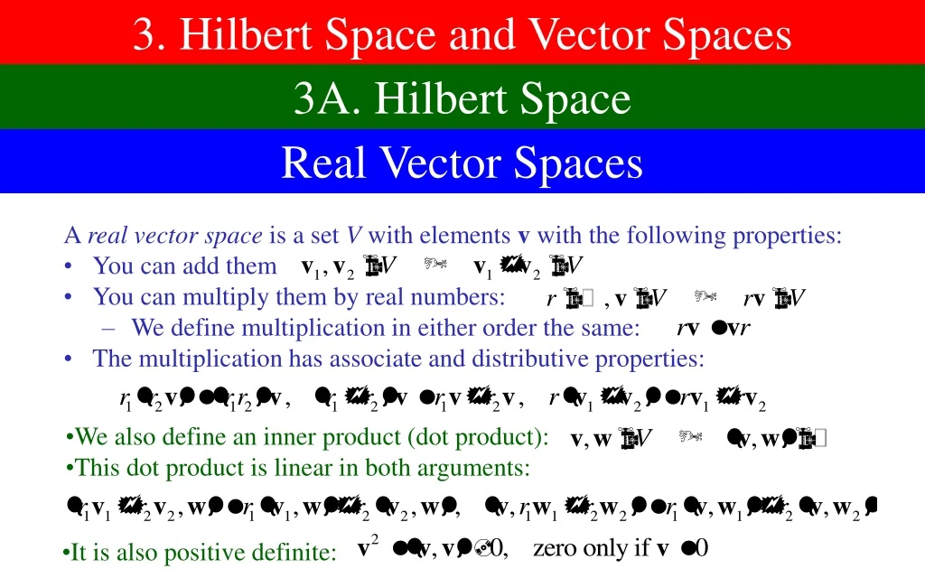
3. Hilbert Space and Vector Spaces 3A. Hilbert Space Real Vector Spaces A real vector space is a set Vwith elements vwith the following properties: • You can add them • You can multiply them by real numbers: • We define multiplication in either order the same: • The multiplication has associate and distributive properties: • We also define an inner product (dot product): • This dot product is linear in both arguments: • It is also positive definite:
Inner Product for Wave Functions • Consider wave functions at a specific time • Define the inner product of two wave functions: • This inner product is linear in its second argument and anti-linear in the first: • It is also positive definite: • Some other properties can be proven using just these two properties: • Proof complicated in general: • Schwartz inequality (homework):
Hilbert Space • We are especially interested in normalized wave functions Hilbert Space, denoted,is the set of wave functions satisfying Hilbert space is a complex vector space with a positive definite inner product • You can add wave functions: • You can multiply them by complex numbers: • Let’s prove closure under addition: positive
Extended and Restricted Hilbert spaces • Hilbert space has only the restriction • Sometimes, we wish to consider wave functions that do not fit this restriction, like eikr • In this case, we are looking at a superspace of Hilbert space • Sometimes, we want to consider more restrictive constraints • |(r)| < • (r) continuous • ’(r) exists, ’’(r) exists … • In this case, we are looking at a subspaceof Hilbert space • These mathematical niceties won’t concerns us much
3B. Dirac Notation and Covectors Vectors/Kets • A wave function and its Fourier transform contain equivalent information • There are other ways to denote a wave function as well: • We might want to consider cases not denoted just by a wave function • Spin • Multiple particles • Indefinite number of particles • To keep our notation as general as possible, we will denote this information as an abstract vector, and clarify it by drawing a ket symbol around it:
Covectors / Bras • A covector, such as f is a linear mappingfrom vectors to complex numbers • Linear means: • Dirac drew a bra around a covector to signal that it’s a covector • When you put a bra with a ket, you get a bracket • The extra bar is deleted for brevity Some examples of covectors/bras: • The position bra r| • The momentum bra k| • For any | , define | by
Covectors as a Vector Space • For any two covectors f1| and f2| and any two complex numbers c1 and c2, define the covector by • Covectors form a vector space * as well • In fact, there is a one-to one-correspondence between vectors and covectors • Mathematically, this means the two vector spaces are the same, = * • The process of turning a bra into its corresponding ket and vice-versa is called Hermitian Conjugation and is denoted by a dagger
Sample Problem What are the corresponding kets (wave functions) for the position and momentum bras?
Hermitian Conjugation and Complex Numbers • Consider the Hermitian Conjugate of a linear combination: • This is defined by how it acts on an arbitrary ket: • Sums remain sums under Hermitian conjugation • But Hermitian conjugation takes the complex conjugate of complex numbers
3C. Coordinate Bases What’s a Coordinate Basis? • In 3D space, it is common to write vectors in terms of components: • In a complex vector space, we would similarly like to write • It is complete if every vector can be written this way • It is independent if there is no non-trivial way to write the zero ket this way • It is orthogonalif the inner product between any distinct pair vanishes • It is orthonormal if:
Making an Orthonormal Basis • Any complete basis can be made into a complete, independent, orthonormal basis • To make it independent, throw out redundant basis vectors: • To make it orthogonal, iteratively produce new vectors orthogonal to each other • To make it orthonormal, normalize them • Our basis is now:
Pulling out the Coefficients • In general, given | and a basis, we wouldlike to find the complex numbers ci such that • Assuming the basis is complete, this can always be done, but actually doing it may be difficult • For an orthonormal basis, this is easy. Act on | with n|: Dimensionality of a Vector Space • The dimensionality of a vector space is the number N of basis vectors in a complete, independent basis • Usually infinity for us
Continuous Bases • Sometimes, it is more useful to work with bases that are labeled by real numbers rather than discrete integers • Then a general ket can be written as • An orthonormal basis would have the property: • The coefficient functions are easily determined: • Some examples in 3D of complete continuous bases: • It is also common to simultaneously use mixed continuous and discrete bases
3D. Operators Operators and Linear Operators • An operator is anything that maps vectors to vectors: • Usually, omit the parentheses • I will (usually) denote operators by capital letters A • We will focus almost exclusively on linear operators: • When I say “operator”, linear is implied • Operators themselves form a vector space: • Technically, this space is *
Examples of Operators • The identity operator 1: • I will rarely bold the 1 • The position operators R = (X,Y,Z), which multiply by the coordinate: • The momentum operators: P = (Px,Py,Pz) which take a derivative: • The Hamiltonian operator: • The Parity operator , which reflects the wave function through the origin: • For any ket |1 and bra 2|, define |12| by
The completeness relation • Let {|i} be a complete orthonormal basis • Consider the following expression: • To figure out what this is, let it act on an arbitrary ket | • We already know: • Therefore: • Since this is true for all |,
Operators acting on covectors (bras) • We normally think of operators acting on vectors to produce vectors: • Operators can also act on covectors to produce covectors • Logically this could be written as A(|), but instead we write this as • This is defined by how we it acts on an arbitrary vector: • Pretty much ignore parentheses • We can just as easily define an operator by how it acts on covectors as on vectors
Multiplying Operators • The product of two operators A and B is defined by • From this property, you can prove the associative property for operators: • Bottom line: Ignore the parentheses: • You can also show the distributive law: • Operator multiplication is usually not commutative
3E. Commutators Definition of the Commutator: • Usually, two operators do not commute: • Define the commutator of two operators A and B by • Warning: avoid using [] as grouping when doing commutators Let’s work out the commutator of X and Px • To do so, let X and Px act on an arbitrary wave function :
Some Simple Commutators: • Generalize: • Some other simple ones: • Some easy to prove identities to help you get more commutators:
Sample Problem The angular momentum operators are defined as L = R P. Find the commutator of Lz with all components of R.
3F. Hermitian Adjoints of Operators Definition of the Adjoint of an Operator: • Let A be an arbitrary operator. Define the HermitianadjointA† by where | = |† • This is a linear operator: • A very useful formula: • From this, easy to show:
Conjugates of products of operators • What is (AB)†? General Rules for Finding Adjoints of Expressions: • For sums or differences, treat each term separately • For things that are multiplied (bras, kets, operators), reverse the order • Replace A by A† for each operator • Replace bras kets, | | • Replace complex numbers c by their complex conjugates
Sample Problem Find the Hermitianadjoint of the equation: • Each term in the sum is treated separately • Reverse the order of everything multiplied • Adjoint everything • Did we do it right? • Answer: both are correct • Warning: Don’t reverse the order of labels inside a ket
Hermitian and Unitary Operators • A Hermitian operator A is one such that • A Unitary operator U is one such that • Proving one of these is sufficient • Generally, easiest to prove by inserting an arbitrary ket and bra: • For Hermitian, equivalent to • Sufficient (and sometimes easier) to prove it with basis vectors:
Examples of Hermitian Operators: • The three position operators: • The three momentum operators: • The Hamiltonian
Examples of Unitary Operators • Define the translation operators by howthey translate the position basis vectors: • Taking the Hermitian conjugate • We therefore have: • Define the rotation operators by howthey rotate the position basis vectors: • Where is a 33 matrix satisfying • We therefore have:
Sample Problem If | is normalized and U is unitary, show that U | is normalized. • U | is normalized • |H | is real Sample Problem If H is Hermition, show that |H | is real
3G. Matrix Notation Matrices for Vectors and Covectors • Suppose we have an orthonormal basis {|1, |2, |3, …} • It is common to write vectors |v by simply listing their components • Put the components vitogether into a column matrix • A covector w| can also be written as a list of numbers • Put the components together into a row matrix: • The inner product is then simply matrix multiplication
Matrices for Operators For an arbitrary operator A: • Write A then as a square matrix: • Any manipulation of operators, bras, and kets can be done with matrices
Why Matrix Notation? • Often easier to understand if we think of bras, kets, operators as concrete matrices, rather than abstract objects • Even though our matrices are usually infinite dimensional, sometimes we can work with just a finite subspace, making them finite • In such cases, computers are great at manipulating matrices
Sample Problem For two spin- ½ particles, the spin stateshave four orthonormal basis states: The operator S2, acting on these states, yields Write S2 as a matrix in this basis. • First, pick an order for your basis states:
Hermitian Conjugates in Matrix Notation For a vector and its corresponding covector, • So, if thought of as a matrix, | becomes | bychanging the column into a row and complex conjugating • For an operator: • For complex numbers, Hermitian conjugation means complex conjugation • General rule: Turn rows columns and complex conjugate
Announcements ASSIGNMENTS DayReadHomework Today 3H, 3I 3.3 Wednesday 4A, 4B, 4C 3.4, 3.5 Friday 4D, 4E 3.6 All homework returned On the web: • Chapter 3 Slides • Chapter 2 Homework Solutions 9/15
Changing Bases (1) All the components of a vector, covector, or operator, depend on basis {|i} What if we decide to change to a new orthonormal basis {|’i}? • Define the conversion matrix: • This is a unitary matrix: • Note that each column of V is components of |’i in the unprimed basis Completeness
Changing Bases (2) We can now use V to convert a vector, covector, or operator • Vectors: • Covectors: • Operators: • Note: The primes don’t mean new objects, but the same old objects in a new basis
3H. Eigenvectors and Eigenvalues Definition, and some properties • An eigenvector of an operator A is a non-zero vector |v such that where a is a complex number called an eigenvalue • If |v is an eigenvector, so is c|v • We can normalize eigenvectors when we want to • Eigenvectors of Hermitian operators are real: • Eigenvectors of Unitary operators are complex numbers of magnitude one real real
Orthogonality of Eigenvectors • Hermitian operators can act equally well to the left or to the right on eigenvectors • Let |v1 and |v2 be eigenvectors of A with distinct eigenvalues • Then |v1 and |v2 will be orthogonal to each other The same property applies to Unitary operators U • Let |v1 and |v2 be eigenvectors of Uwith distinct eigenvalues • Recall: • We see that • Consider the expression:
Observables and Basis Sets Suppose that the eigenvectors of a Hermitian operator A form a complete set (mathematically, they span the space), so that we can always write: • This can always be done in finite dimensional space, often in infinite • A Hermitian operator with this property is called an observable Suppose we start with a complete set of eigenstates {|n} • Throw out any redundant ones • Construct an orthogonal basisset by the usual procedure: • Note that states with different eigenvalues don’t mix, so stilleigenstates • Now make them orthonormalby the usual procedure: • Still eigenstates! • We end up with an orthonormal basis set which are eigenstates of A
Labelling Basis States • When we choose a basis set that are eigenvalues of observable A, often label them by their eigenvalues • If we work in this bases, the matrix for A will be diagonal • Switching to this basis is called diagonalizing A • Let B be another observablethat commutes with A, so • If you act on any eigenstate of A with B, it is stillan eigenstate of A: • This implies that B will be block diagonal • When you find eigenstates of B, they will exist justwithin these subspaces with the same A eigenvalues • You can label them by both their eigenvalues under A and B
Complete Sets of Commuting Observables • We can continue this procedure, until eventually our states are uniquely labeled by their eigenvalues • The observables you are using are called a complete set of commuting observables • They must all commute with each other • Eigenstates can be labelled just by their eigenvalues Why is this a good idea? • Oddly, making the requirements more stringentcan make them easier to find • Think of an animal whose nameends in -ant • Often, the eigenvalues correspond to physically measurable quantities • In particular, the Hamiltonian is often chosen as one of the observables that has a trunk
3H. Finding Eigenvalues and Eigenvectors How to find Eigenvalues • Suppose an operator is given in matrix form • How can we find its eigenvectors and eigenvectors? • We want to solve: • Rewrite this as: • This is N equations in N unknowns • Generally has a unique solution: |v = 0 • Unless det(A – 1) = 0 ! To find eigenvalues, solve det(A – 1) = 0 • This is an N’th order polynomial • It has exactly N complex roots, thoughnot necessarily distinct • For Hermitian matrices, these roots will be real
Procedure for Eigenvalues and Eigenvectors To find the eigenvalues and orthonormal eigenvectors of operator A: • First find roots of det(A – 1) = 0 • This produces N eigenvalues {n} • Then, for each eigenvalue n: • Solve the equation A|vn = n|vn • If you have any degenerate eigenvalues n, you may have to be careful to keep them orthogonal • You then need to normalize them: vn|vn = 1 To change basis to the new basis vectors • Make the basis transformationmatrix V from the eigenvectors |vn • You can then use this to transformvectors, covectors or operators to the new basis • In particular, the operator A will be diagonaland will have the eigenvalues on the diagonal • You don’t need to calculate it
Shortcuts for Eigenvalues and Eigenvectors • If a matrix is already diagonal, theeigenvalues and eigenvectors are trivial • The eigenvalues are the values on the diagonal • The eigenvectors are the unit vectors in this basis • If a matrix is block diagonal, you can divide it into two(or more) smaller and easier problems • If there is a common factor in an operator, take it out • Matrix without c has identicalnormalized eigenvectors • Eigenvalues are identical exceptmultiplied by c
Sample Problem (1) For the S2 matrix found before, (1) Find the eigenvalues and orthonormal eigenvectors (2) Find the matrix V that relates the new basis to the old, and demonstrate explicitly that V†S2V is now diagonal (3) Write the state |2 = |+– in terms of the eigenvector basis. • Take the common factor of 2 out. • Note that it is block diagonal • Two of the eigenvectors andeigenvalues are now trivial • All that’s left is the middle
Sample Problem (2) (1) Find the eigenvalues and orthonormal eigenvectors . . . • Solve the equation det(S2 - 1) = 0 • For each eigenvalue, solve S2|v = |v • = 0: • = 2: • The eigenvalues of S2 will be 2 times these, or 0 and 22
Sample Problem (3) (1) Find the eigenvalues and orthonormal eigenvectors (2) Find the matrix V that relates the new basis to the old, . . .
Sample Problem (4) . . .and demonstrate explicitly that V†S2V is now diagonal
Sample Problem (5) (3) Write the state |2 = |+– in terms of the eigenvector basis.