Download
1 / 11
110 likes | 404 Views
2. Quantum Mechanics and Vector Spaces. 2.1 Physics of Quantum mechanics Principle of superposition Measurements 2.2 Redundant mathematical structure 2.3 Time evolution The Schr ödinger equation Time evolution operator Example: Electron Spin Precession.

E N D
2. Quantum Mechanics and Vector Spaces 2.1 Physics of Quantum mechanics • Principle of superposition • Measurements 2.2 Redundant mathematical structure 2.3 Time evolution • The Schrödinger equation • Time evolution operator • Example: Electron Spin Precession
We can produce interference between different components of a quantum state, e.g. Two-slit experiment photons, electrons, buckyballs (C60)… Bragg diffraction: interference between particles reflected from different planes in a crystal Photons, electrons, neutrons, H2 molecules Superconducting Quantum Interference Devices (SQUIDS): interference between electric currents travelling around loop in opposite directions. “The most beautiful experiment in physics” …according to Physics World readers (2002) 2.1.1 Principle of Superposition Credit: Tonomura et al, Hitachi Corp.
SG−x SG x SG x Interference experiments | | SG−x | SG z φ | | Feynman thought experiment • Destructive interference genuine wave-like superposition, not just addition of probabilities. • Interference pattern depends on both relative amplitude and ‘phase difference’ between components represent as complex amplitude. • Interference always seen whenever theory predicts it should be detectable. • Physical states can be added and multiplied by complex numbers, i.e. they have the structure of a vector space.
Why not stick with wave functions? • Don’t take ‘vector’ too seriously • …it’s a metaphor • Really a general theory of “superposables” • So you can always think of waves instead if that helps. • Often we’re interested in quantum numbers, not the wave pattern: vector approach avoids calculating wave functions when not needed. • Wave function picture incomplete: • If you know ψ(r) you know everything about: • position, momentum, KE, orbital angular momentum • …but nothing about spin (+ other more obscure quantities) Vector space allows us to easily include spin.
Only certain results found in quantum measurement: some quantities quantized (ang. mom., atomic energy levels) some continuous (position, momentum of a free particle). We can prepare quantum states that will definitely give any allowed result for a quantized observable an arbitrarily small spread for continuous observables. There is ‘something there’ to measure. SG z Ag SG z SG z Ag 2.1.2 Measurements
SG−z SG z SG z Measurement (continued) | SG−z SG z Ag | • If we superpose definite states of a given observable, & measure the same observable, we randomly get one of the superposed values—never an ‘intermediate’ result. • Probability of result a, Prob(a) |amplitude|2 in superposition. • We always get some result: Probs = 1.
Represent states of definite results (eigenstates) as a set of orthonormal basis vectors. Represent physical states as normalised vectors. Probability amplitude for result ai from state ψ: ci = ai |ψ. zero amplitude to get anything but ai in “definite ai” state. Use projectors instead, if degenerate. General state can always be decomposed into a superposition: Sum of probabilities = 1 is Pythagoras rule in N-D vector space! 1 cz|z |ψ cx|x cy|y Mathematical model
2.2 Redundant Mathematical Structure • A mathematical model for a physical process may contain things that don’t have any physical meaning. • e.g. in electromagnetism, vector potential is undetermined up to a gauge change: A A + • Bad thing? May make the maths much easier! • In QM, physical states are represented by normalised vectors: • Ambiguous up to factor of eiθ, i.e. |ψ and eiθ|ψ represent the same state. • Normalised vectors do not make a vector space—maths requires vectors of all lengths. • Really, physical state equivalent to a ‘ray’ through the origin: normalisation is a convention as we could write: • Vectors of a particular length & phase needed when analysing a vector into a superposition.
Redundancy (continued) • Vector space may include unphysical vectors: • all those with infinite energy, i.e. outside the domain of the energy operator, Ĥ, (e.g. discontinuous wave functions). • Should other operators (x ? p ?) have finite expected values? • Do all possible self-adjoint operators represent physical observables? • In practice, no: we only need a few dozen. • In theory, no: some self-adjoint ops represent things disallowed by ‘superselection’ — e.g. real particles are either bosons or fermions, not some mixture.