Download
1 / 32
430 likes | 1.15k Views
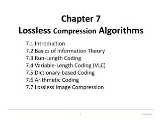
Fundamentals of Multimedia Chapter 7 Lossless Compression Algorithms Ze-Nian Li and Mark S. Drew. 건국대학교 인터넷미디어공학부 임 창 훈. Outline. 7.1 Introduction 7.2 Basics of Information Theory 7.3 Run-length Coding 7.4 Variable-length Coding 7.4.1 Shannon-Fano Algorithm 7.4.2 Huffman Coding

E N D
Fundamentals of MultimediaChapter 7Lossless Compression AlgorithmsZe-Nian Li and Mark S. Drew 건국대학교 인터넷미디어공학부 임 창 훈
Outline 7.1 Introduction 7.2 Basics of Information Theory 7.3 Run-length Coding 7.4 Variable-length Coding 7.4.1 Shannon-Fano Algorithm 7.4.2 Huffman Coding 7.6 Arithmetic Coding Li & Drew; 인터넷미디어공학부 임창훈
2.1 Introduction • Compression: the process of coding that will effectively reduce the total number of bits needed to represent certain information. General data compression scheme Li & Drew; 인터넷미디어공학부 임창훈
If the compression and decompression processes induce no information loss, then the compression scheme is lossless; otherwise, it is lossy. • Compression ratio: compression ratio =B0 / B1 B0 : number of bits before compression B1 : number of bits after compression Li & Drew; 인터넷미디어공학부 임창훈
7.2 Basics of Information Theory • The entropyof an information sourcewith alphabet S = {s1, s2, …, sn} pi: probability that symbol siwill occur in S. log2(1/pi) : the amount of information contained in si, which corresponds to the number of bits needed to encode si. Li & Drew; 인터넷미디어공학부 임창훈
Distribution of Gray-Level Intensities Fig. 7.2 Histograms for two gray-level images. Fig. 7.2(a) shows the histogram of an image with uniformdistribution of gray-level intensities, i.e., pi= 1/256 for all i. Hence, the entropy of this image is: log2 256 = 8 Li & Drew; 인터넷미디어공학부 임창훈
Entropy and Code Length • The entropy H(S) is a weighted-sum of terms log2(1/pi) • Hence it represents the average amount of information contained per symbol in the source S. • The entropy H(S) specifies the lower bound for the average number of bits to code each symbol in S, i.e., - the average length (in bits) of the codewords produced by the encoder Li & Drew; 인터넷미디어공학부 임창훈
7.3 Run-Length Coding • Memoryless Source: an information source that is independently distributed. Namely, the value of the current symbol does not depend on the values of the previously appeared symbols. • Instead of assuming memoryless source, Run-Length Coding (RLC)exploits memory present in the information source. Li & Drew; 인터넷미디어공학부 임창훈
7.4 Variable-Length Coding (VLC) • Shannon-Fano Algorithm : a top-down approach • Sort the symbols according to the frequency count (probability) of their occurrences. 2. Recursively divide the symbols into two parts, each with approximately the same number of counts, until all parts contain only one symbol. An Example: coding of “HELLO“ Frequency count of the symbols in "HELLO". Li & Drew; 인터넷미디어공학부 임창훈
Shannon-Fano Algorithm Coding tree for HELLO by the Shannon-Fano algorithm Li & Drew; 인터넷미디어공학부 임창훈
Shannon-Fano Algorithm One result of performing the Shannon-Fano algorithm on HELLO Li & Drew; 인터넷미디어공학부 임창훈
Shannon-Fano Algorithm Another coding tree for HELLO by the Shannon-Fano algorithm Li & Drew; 인터넷미디어공학부 임창훈
Shannon-Fano Algorithm Another result of performing the Shannon-Fano algorithm on HELLO Li & Drew; 인터넷미디어공학부 임창훈
7.4.2 Huffman Coding • Huffman coding Algorithm: a bottom-up approach • Initialization: Put all symbols on a list sorted according to their frequency counts (probability). 2. Repeat until the list has only one symbol left: • From the list pick two symbols with the lowest frequency counts (probability). Form a Huffman subtree that has these two symbols as child nodes and create a parent node. (b) Assign the sum of the children's frequency counts to the parent and insert it into the list such that the order is maintained. (c) Delete the children from the list. 3. Assign a codeword for each leaf based on the path from the root. Li & Drew; 인터넷미디어공학부 임창훈
Huffman Coding Coding tree for HELLO by the Huffman algorithm Li & Drew; 인터넷미디어공학부 임창훈
Huffman Coding • New symbols P1, P2, P3 are created to refer to the parent nodes in the Huffman coding tree. The contents in the list are illustrated below: Li & Drew; 인터넷미디어공학부 임창훈
Properties of Huffman Coding • Unique Prefix Property: No Huffman code is a prefix of any other Huffman code - precludes any ambiguity in decoding. Li & Drew; 인터넷미디어공학부 임창훈
2. Optimality: minimum redundancy code – proved optimal for a given data model (i.e., a given probability distribution): • The two least frequent symbols will have the same length for their Huffman codes, differing only at the last bit. • Symbols that occur more frequently (higher probability) will have shorter Huffman codes than symbols that occur less frequently. • The average code length for an information source S is strictly less than η+ 1. Li & Drew; 인터넷미디어공학부 임창훈
7.6 Arithmetic Coding • Arithmetic coding is a more modern coding method that usually out-performs Huffman coding. • Huffman coding assigns each symbol a codeword which has an integral bit length. Arithmetic coding can treat the whole message as one unit. • A message is represented by a half-open interval [a. b) where aand bare real numbers between 0 and 1. Li & Drew; 인터넷미디어공학부 임창훈
Initially, the interval is [0, 1). • When the message becomes longer, the length of the interval shortens and the number of bits needed to represent the interval increases. Li & Drew; 인터넷미디어공학부 임창훈
Arithmetic Coding Arithmetic coding encoder Li & Drew; 인터넷미디어공학부 임창훈
Example: Encoding in Arithmetic Coding Arithmetic Coding: Encode Symbols CAEE$ (a) Probability distribution of symbols. Li & Drew; 인터넷미디어공학부 임창훈
(b) Graphical display of shrinking ranges Li & Drew; 인터넷미디어공학부 임창훈
(c) New low, high, and range generated. Li & Drew; 인터넷미디어공학부 임창훈
Generating codeword for encoder The final step in Arithmetic encoding calls for the generation of a number that falls within the range [low; high). The above algorithm will ensure that the shortest binary codeword is found. Li & Drew; 인터넷미디어공학부 임창훈
Arithmetic coding decoder Li & Drew; 인터넷미디어공학부 임창훈
Arithmetic coding: decode symbols CAEE$ Li & Drew; 인터넷미디어공학부 임창훈
7.7 Lossless Image Compression • Approaches of Differential Coding of Images: Given an original image I(x, y), using a simple difference operator we can define a difference image d(x, y) as follows: d(x, y) = I(x, y) − I(x − 1, y) or use the discrete version of the 2-D Laplacian operator to define a difference image d(x, y) as d(x, y) = 4I(x, y) − I(x, y − 1) − I(x, y +1) − I(x+1, y) − I(x−1, y) • Due to spatial redundancy existed in normal images I, the difference image dwill have a narrower histogram and hence a smaller entropy. Li & Drew; 인터넷미디어공학부 임창훈
Distributions for Original versus Derivative Images. (a): Original gray-level image (b) Partial derivative image; (c): Histograms for original (d) Histogram for derivative images. Li & Drew; 인터넷미디어공학부 임창훈
Lossless JPEG • Lossless JPEG: A special case of the JPEG image compression. • The Predictive method • Forming a differential prediction: A predictor combines the values of up to three neighboring pixels as the predicted value for the current pixel, indicated by `X' in Fig. 7.10. 2.Encoding:The encoder compares the prediction with the actual pixel value at the position `X' and encodes the difference using one of the lossless compression techniques we have discussed, e.g., the Huffman coding scheme. Li & Drew; 인터넷미디어공학부 임창훈
Fig. 7.10: Neighboring Pixels for Predictors in Lossless JPEG. Note: Any of A, B, or C has already been decoded before it is used in the predictor, on the decoder side of an encode- decode cycle. Li & Drew; 인터넷미디어공학부 임창훈
Predictors for Lossless JPEG Li & Drew; 인터넷미디어공학부 임창훈