Lossless Compression
Lossless Compression. Lossless Compression Overview. Algorithms that allow for the exact pre-compressed data to be constructed from the compressed data Used when no loss of data can be allowed Text compression Executable compression General file compression (ZIP, RAR)

Lossless Compression
E N D
Presentation Transcript
Lossless Compression Overview • Algorithms that allow for the exact pre-compressed data to be constructed from the compressed data • Used when no loss of data can be allowed • Text compression • Executable compression • General file compression (ZIP, RAR) • Can’t guarantee that all data sets will be made smaller • Compression must make a result for any particular data set unique in order to allow for perfect reconstruction of the original data • Can’t make a unique result for all data sets if all data sets are made smaller
Proof of Compression Problem • Let S(n) be the number of files of at the most size n bits • S(n) = 1+2+4+8…+2n = 2n+1-1 • Now take S(n-1) (the largest smaller file you could make • S(n-1) = 1+2+4+8…+2n-1 = 2n-1 • Naturally, 2n-1 is smaller than 2n+1-, so each file of size n or less can’t be uniquely mapped to a file of size n-1 or less
Helping Out Lossless Compression • Highly repetitive data allows for a higher degree of compression. • Modifying your data set to create a more repetitive data set would result in a more compressed result. • Modification must be reversable to allow for lossless compression • BWT (Burrows-Wheeler transform), also called Block Sorting, provides the ability to modify your data in to a more repetitive form, as well as allowing for easy reversal.
Doing the BWT • The process for the BWT is as follows: • The data set has an arbitrary character appended to the end, and is pointed to to represent the end of the data set • A list of all possible rotations of the data set is created, with each rotation being thought of as a row in a n x n matrix, where n is the number of characters in the data set • The rows of the table are sorted alphabetically • The last column of the table is then taken as your new data set, containing new highly repetitive data
BWT Example • Take the simple data set: • STPLSRQTLTMTPSQ* where * is the end of data pointer Taking the last column of the sorted list the data set becomes PTTTTRSSPL*QLSMQ, a much more repetitive data set
Reversing the BWT • The ability to reverse the BWT is crucial to allowing for lossless data compression • The process by which it is done is as follows: • Create a new empty list (n x n) • Loop n times • Insert the data set in to the left most column • Sort the list • Take the row that ends with the end of data character, this is your original data set
Example of the BWT reversal • Using our transformed data set PTTTTRSSPL*QLSMQ: Taking the line that ends with the termination character, we get our original data: STPLSRQTLTMTPSQ*
LZ Transformations • Two forms, LZ77 and LZ78, developed by Abraham Lempel and Jacob Ziv in 1977 and 1978 respectively. • Used mainly for text compression. • LZ77 keeps a window of previously viewed data and compares the current data • Compressed data is represented as an index in to the window, and a length • If no match can be found in the window, the text gets tagged as literal data, not compressed data • LZ78, and the updated LZW, maintain a dictionary of code words and compare the data to the dictionary • If the current data is in the dictionary, it is replaced by that entry’s value. • If the data is not in the dictionary, it is maintained in the compressed file as is, but is added to the dictionary as a new entry. • The larger the input file, the more the dictionary grows, creating a higher degree of compression • Exact dictionary can be recreated on decompression, needing no dictionary to be passed with data. • For use with ASCII, each symbol and dictionary entry will need its own number, so more than 8 bits will be needed per value (literal or dictionary entry).
LZW compression • The algorithm for compression is as follows: • Maintain 2 variables w and k. • Initially set w to NULL • While (not EOF) • Read a character • If wk exists in the dictionary, set w to wk and loop • If not, output w and add wk to the dictionary. • Set w to k and loop
LZW compression example Result: I.am.who.[256][258][257]nd[264][257][259]not[260][262][270][266][273]t Original text: 39 characters of 8 bits 312 bits total Compressed text:26 characters of 9 bits 234 bits total Savings of 25% Larger data sets would produce more entries in the dictionary, making for even higher compression ratios • Sample data: I.am.who.I.am.and.I.am.not.who.I.am.not
LZW decompression • The LZW decompression algorithm is as follows: • read in a character k and output it, setting it to w • while (not EOF) • read in character k • set entry to dictionary entry for k if it exists, set to k otherwise • add w + the first character of entry to dictionary • set w to w+entry and loop
LZW decompression example The result is the original data: I.am.who.I.am.and.I.am.not.who.I.am.not The result is created entirely from the sent message, so there is no need for any dictionary to be sent. • Using out compressed data: I.am.who.[256][258][257]nd[264][257][259]not[260][262][270][266][273]t
Huffman coding • Developed in 1951 by David Huffman, an MIT student, as a paper to get out of his Information Theory final exam • Uses a frequency sorted binary tree to produce bit codes for symbols • Based on an alphabet with a set weight applied to how likely a character is to arise • Results are prefix free, meaning that no codeword is the prefix for any other codeword • The algorithm takes in an alphabet as an array (a), and the cost of each element in the alphabet (c) where c[i] = cost(a[i]) • The algorithm produces an array of bit codes for the alphabet (h) where h[i] is the codeword for a[i] • The algorithm uses a min heap to create the tree. • left children are considered a 0 bit and right children are considered a 1 bit • After tree is created a traversal of the tree can be used to retrieve the bit codes
Huffman Coding algorithm • create a leaf node for all alphabet entries. The node contains the character and the character’s weight • Put all nodes on to a min heap sorted by weight • While there is more than one node left on the heap • remove the top 2 nodes from the heap (sifting up after each removal) • create a new internal node with the 2 nodes as it’s children and a weight of the sum of the 2 node’s weights • add the new node to the heap • When only one node remains in the heap, that is the root node • A traversal of the tree will result in the bit codes for each character
Huffman Coding Example • Given an alphabet with the following properties: Initial Heap: 1st 2 items off heap are c and d. A new internal node (I1) is created and put on heap After 1st removes 1st 2 items off heap are b and I1. A new internal node (I2) is created and put on heap After 2nd removes 1st 2 items off heap are a and I2. A new internal node (I3) is created and put on heap After 3rd removes e and I3 come off heap. A new internal node (I4) is created and put on heap After 4th removes Only 1 node left on heap, it becomes the root
Huffman Coding example tree • This is the tree resulting from the previous example I4 0 1 e I3 Either a weight convention can be used for the alphabet, in which case the bit codes can be generated at the receiving end, or the weights can be dependant on the actual data, which will give more accurate results, but require the bit codes to be sent with the transmission 0 1 I2 a 0 1 I3 b 1 0 c d