Stat 31, Section 1, Last Time
630 likes | 785 Views
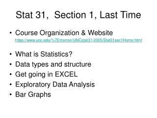
Stat 31, Section 1, Last Time. 2 Sample Inference Paired Differences Apply 1 sample methods to differences Unmatched Samples Requires deeper methods Work through TTEST. Reading In Textbook. Approximate Reading for Today’s Material: Pages 485-504, 536-549

Stat 31, Section 1, Last Time
E N D
Presentation Transcript
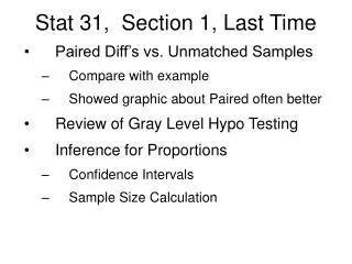
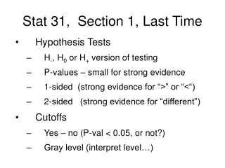
Stat 31, Section 1, Last Time • 2 Sample Inference • Paired Differences • Apply 1 sample methods to differences • Unmatched Samples • Requires deeper methods • Work through TTEST
Reading In Textbook Approximate Reading for Today’s Material: Pages 485-504, 536-549 Approximate Reading for Next Class: Pages 555-566, 582-611
Midterm II Coming on Tuesday, April 10 Think about: • Sheet of Formulas • Again single 8 ½ x 11 sheet • New, since now more formulas • Redoing HW… • Asking about those not understood • Will schedule Extra Office Hours • Midterm II not cumulative
2 Sample Hypo Testing Comparison of Paired vs. Unmatched Cases Notes: • Can always use unmatched procedure • Just ignore matching… • Advantage to pairing???
2 Sample Hypo Testing Comparison of Paired vs. Unmatched Cases • Advantage to Pairing??? • Recall previous example: Old Textbook 7.32 • Matched Paired P-value = 1.87 x 10⁻⁵ • Unmatched P-value = 3.95 x 10⁻⁶ • Unmatched better!?! (can happen)
2 Sample Hypo Testing Comparison of Paired vs. Unmatched Cases • Advantage to Pairing??? Happens when “variation of diff’s”, , is smaller than “full sample variation” I.e. (whether this happens depends on data)
Paired vs. Unmatched Sampling Class Example 29: A new drug is being tested that should boost white blood cell count following chemo-therapy. For a set of 4 patients, it was not administered (as a control) for the 1st round of chemotherapy, and then the new drug was tried after the 2nd round of chemotherapy. White blood cell counts were measured one week after each round of chemotherapy.
Paired vs. Unmatched Sampling Class Example 29: The resulting white blood cell counts were:
Paired vs. Unmatched Sampling Class Example 29: Does the new drug seem to reduce white blood cell counts well enough to be studied further? • Seems to be some improvement • But is it statistically significant? • Only 4 patients…
Paired vs. Unmatched Sampling Let: = Average Blood c’nts w/out drug = Average Blood c’nts with drug Set up: (want strong evidence of improvement)
Paired vs. Unmatched Sampling Class Example 29: http://stat-or.unc.edu/webspace/postscript/marron/Teaching/stor155-2007/Stor155Eg29.xls Results: • Matched Pair P-val = 0.00813 • Very strong evidence of improvement • Unmatched P-val = 0.295 • Not statistically significant
Paired vs. Unmatched Sampling Class Example 29: http://stat-or.unc.edu/webspace/postscript/marron/Teaching/stor155-2007/Stor155Eg29.xls Conclusions: • Paired Sampling can give better results • When diff’ing reduces variation • Often happens for careful matching
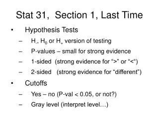
Review Gray Level Testing • Seems some uncertainty about this… • Go over previous examples, with links • Recall main ideas • 0.1 < P-value : no strong evidence • 0.01 < P-value < 0.1: somewhat strong evidence (use words to indicate strength) • P-Value < 0.01: very strong evidence
Review Gray Level Testing Some examples of words, in the gray level region: • P-value ~ 0.09: “mild evidence, but perhaps something is there” • P-value ~ 0.07: “not strong evidence, but some indication”
Review Gray Level Testing Some examples of words: • P-Value ~ 0.05: “close to the boundary of strong evidence” • P-value ~ 0.03: “fairly strong evidence” • P-value ~ 0.02: “close to being very strong evidence”
Review Gray Level Testing Some earlier class examples: March 20, page 18: P-value of 0.094 “Quite weak evidence, i.e. only a mild suggestion”
Review Gray Level Testing March 20, page 44: P-value of 0.031 “Pretty strong evidence” P-value of 0.062 “Not very strong, but some indication of something there”
Review Gray Level Testing March 22, page 32, HW 6.82: P-value of 0.382 “No evidence” P-value of 0.171 “No evidence” P-value of 0.0013 “Very strong Evidence”
Review Gray Level Testing March 22, page 32, HW 6.84: P-value of 0.0505, “Close to boundary of strong evidence, but not quite there” P-value of 0.0495 “Just over boundary of strong evidence, but very close”
Review Gray Level Testing March 27, page 44, HW 7.16: P-value of 0.04, “moderately strong evidence” March 27, page 44, HW 7.21: P-value of 0.188 “No evidence”
Review Gray Level Testing March 29, page 16, HW 6.61: P-value of 0.0401, “moderately strong evidence” March 29, page 33, HW 7.27: P-value of 0.739 “No evidence”
Review Gray Level Testing March 29, page 33, HW 7.31: P-value of 0.0001 “Very strong evidence” March 29, page 33, HW 7.41: P-value of 0.00052 “Very strong evidence”
And now for somethingcompletely different…. Another fun movie Thanks to Trent Williamson
Inference for proportions Sec. 8.1: A deeper look (already know some basics, but there are some fine point worth a deeper look) Recall: Counts: Sample Proportions:
Inference for proportions Calculate prob’s with BINOMDIST, but note no BINOMINV, so instead use Normal Approximation Revisit Class Example 20 http://stat-or.unc.edu/webspace/postscript/marron/Teaching/stor155-2007/Stor155Eg20.xls
Inference for proportions Recall Normal Approximation to Binomial: For is approximately is approximately So use NORMINV (and often NORMDIST)
Inference for proportions Main problem: don’t know Solution: Depends on context: CIs or hypothesis tests Different from Normal, since mean and sd are linked, with both depending on , instead of separate .
Inference for proportions Case 1: Margin of Error and CIs: 95% 0.975 So:
Inference for proportions Case 1: Margin of Error and CIs: Continuing problem: Unknown Solution 1: “Best Guess” Replace by
Inference for proportions Solution 2: “Conservative” Idea: make sd (and thus m) as large as possible (makes no sense for Normal) zeros at 0 & 1 max at
Inference for proportions Solution 1: “Conservative” Can check by calculus so Thus