Cooperative Optimization and Navigation Problems
450 likes | 471 Views
Explore bio-inspired trajectory optimization and language-based navigation for groups of autonomous vehicles. Report detailing progress on event-driven communication, local pursuit algorithm, and experimental results in pursuit on 5m trajectory.

Cooperative Optimization and Navigation Problems
E N D
Presentation Transcript
Cooperative Optimization and Navigation Problems Dimitrios Hristu-Varsakelis Mechanical Engineering and Institute for Systems Research University of Maryland, College Park http://glue.umd.edu/~hristu hristu@glue.umd.edu Joint work with: M. Egerstedt, S. B. Andersson, C. Shao. P.R. Kumar, P. S. Krishnaprasad,
Ensembles of autonomous vehicles operating on “expansive” terrain. Bio-inspired trajectory optimization Language-based navigation Report on Progress – Event-driven communication Outline
Ensembles of Autonomous Systems • Examples from biology (bees, ants, fish etc.) • Ensembles can accomplish tasks that are impossible for an individual. • Coordination requires thinking about control/communication interactions.
Trajectory optimization without a map • A group of vehicles traveling between a fixed pair of locations • Terrain is unknown - no “global” map. • On-board sensing provides local information about vehicle’s immediate surroundings target vehicle Vn-1 V1 Vn obstacle control station start PROBLEM: Given an initial path between a pair of “start” and “target” locations, find the optimal path connecting that pair, using “local” interactions between vehicles.
Trajectory optimization without a map • A group of vehicles traveling between a fixed pair of locations • Terrain is unknown - no “global” map. • On-board sensing provides local information about vehicle’s immediate surroundings target Vn-1 vehicle V1 obstacle Vn control station start PROBLEM: Given an initial path between a pair of “start” and “target” locations, find the optimal path connecting that pair, using “local” interactions between vehicles.
Local pursuit: A biologically-inspired algorithm k+1 k ... K+2 ... Target ... Start : Initial path : path followed by the k-th vehicle, Theorem (on ): The iterated paths converge to a straight line as [Bruckstein, 92] (on a smooth manifold M): If vehicle separation is sufficiently small, then the iterated paths converge to a geodesic.
Experimental results: with Euclidean metric • A collection of mobile robots with: • Wireless communication between neighbors • Sonar and odometry sensors TARGET START Initial path length ~7m Vehicle separation ~1.5m
Local Pursuit : location of k-th vehicle M : Minimum-length geodesic connecting to Idea: Find optimal trajectory to leader and follow it momentarily.
Pursuit decreases vehicle separation M : Minimum-length geodesic connecting a to b : location of k-th vehicle
Local pursuit for more general optimal control problems Let Given an initial trajectory with Find that minimizes s.t. The k-th vehicle moves as follows: Wait at until t=Δ(κ+1) At time t, “follow the optimal trajectory” from to As , iterated trajectories converge to a local min. for Assumptions: uniqueness, smoothness
Simulation: pursuit on 5m trajectory 0.7m separation
A sub-Riemannian example fixed 5m trajectory 1.5m separation
Summary and Work in Progress • A biologically-inspired trajectory optimization algorithm • - local pursuit forms a “string” of vehicles • - each vehicle uses local information and • communicates with its closest neighbors • Target state and optimal trajectory are unknown • Local convergence • Experiments • Escaping local minima • Comparison with gradient descent methods
Control in a reasonably complex world • The problem of specifying control tasks (e.g. “go to the refrigerator and get the milk”) • Solving motion control problems of adequate complexity • Many interesting systems evolve in environments that are not smooth, simply connected, etc. • Using language primitives to navigate: • Specify control policies • Represent the environment (what parts do we ignore?)
Motion Description Languages Atom: Evolve under until Evaluate Concatenate, encapsulate atoms to form complex strings (plans), e.g. Def: MDLe is the formal language defined by the context free grammar with production rules: N: nonterminals T: terminals S: start symbol ε:empty string Fact: MDLe is context free but not regular
Keep only “interesting” details about how to navigate the world Landmark: L = (M,x) M: map “patch”, x: coordinates Sensor signature: L = Li if s(t) = si(t) for t in [t0,T] Navigation Local navigation: on a given landmark Li Global navigation: between landmarks Symbolic Navigation World M x
Represent only “interesting parts” of the world. G = {L,E} Li : landmarks Eij : {i,j,Gij} Γij: an MDLe program Eij Eji Idea: Replace details locally by a feedback program A directed graph representation of a map
Experiment: indoor navigation Lab 1 Lab 2 Office Partial floor plan of 2nd floor A.V. Williams
Goal: Navigate between three landmarks Experiment, cont’d Front of lab Rear of lab Office
{Lab2toLab1Plan (bumper) (Atom (atIsection 0100) (goAvoid 90 40 20)) (Atom (atIsection 0010) (go 0 0.36)) (Atom (wait ) (align 7 9)) (Atom (atIsection 1000) (goAvoid 0 40 20)) (Atom (atIsection 0100) (go 0 0.36)) (Atom (wait ) (align 3 5)) (Atom (wait 7) (goAvoid 270 40 20)) (Atom (atIsection 1000) (goAvoid 270 40 20)) } Experiment: Example MDLe plans {Lab1toOfficePlan (bumper) (Atom (atIsection 1001) (goAvoid 90 40 20)) (Atom (atIsection 0011) (go 0 0.36)) (Atom (wait ) (align 11 13)) (Atom (atIsection 0100) (goAvoid 180 40 20)) (Atom (wait 10) (rotate -90)) }
Controllers (and MDLe plans) are not always successful. Environmental factors (moving obstacles) System uncertainty (e.g. actuator noise) Associate a probability density function with an MDLe plan Enumerate the MDLe strings associated with an environment graph G = {L,E}, Define Prob. of arriving at by executing from Assumptions: G is a “good” description of the world Sensor model: Incorporating Uncertainty
How do I get to a given landmark ? A prototype navigation problem Information at “time” k Prob. density at time k, given observations up to time k. Probability after evaluating plan and making a new observation: Maximize probability of arriving at a desired landmark in N “steps” Maximize prob. of arrival at a desired landmark with minimum of “steps” Maximize probability of arriving at desired landmark in N “steps”
Example - data with N(0,0.01) actuator noise Example: L2 to L3 (syntax: (ξ,u))
Example: steer to a landmark in N “steps” X0=L1 , XF=L2, N=3 P0|0=[1/3, 1/3, 1/3] Desired success probability set to 95% Evolution of probability density on G
Example: steer to a landmark in N “steps” True and observed landmarks
Example: steer to a landmark in N “steps” Executed Plans
Summary and Ongoing Work • Language-based Control • The motion description language MDLe • “Landmark+instruction”-based descriptions of the world • Optimal navigation via dynamic-programming • Obtaining “nominal” densities for navigation • Software
References: • S. Andersson and D. Hristu-Varsakelis, “Stochastic Language-based Motion Control”, to appear, CDC 2003. • D. Hristu-Varsakelis, M. Egerstedt, P. S. Krishnaprasad, “On the Structural Complexity of the Motion Description Language MDLe”, to appear, CDC 2003. • D. Hristu-Varsakelis and P. R. Kumar, “Interrupt-based feedback control over a shared communication medium”, IEEE CDC 2002. • M. Egerstedt and D. Hristu-Varsakelis, “Observability and Policy Optimization for Mobile Robots”, CDC 2002
Event-Based Stabilization of Ensembles-Users of a Shared Network
Dynamical systems as users of a shared “network” plant G1(s) G2(s) GN(s) … shared medium K1 K2 KN controller • Control of collections of systems with limited communication • A prototype problem in “divided attention”. • N=number of systems in the ensemble • n=max. number of feedback loops that can be closed at any time • How much communication time must be devoted to each system • to guarantee that the collection remains stable? • Can the ensemble be stabilized?
A feedback communication policy • We would like to avoid having to specify the communication policy in advance • (thus the need for memory, clocks) • How much information is needed to implement an event-driven policy? • Let’s define a simple rule for deciding which system(s) should be allowed to use the “network”. • Idea: Close loops corresponding to states that are “furthest” from the origin Ex.: N=3, n=2 . . 0 .
A feedback communication policy Definition: An ensemble is δ-captured if for all i after some time Let’s define a simple rule for deciding which system(s) should be allowed to use the “network”. Idea: Close loops corresponding to states that are “furthest” from the origin Ex.: N=3, n=2 . . 0 . For each system, find a Lyapunov function V( ) such that: (feedback loop closed) (feedback loop open)
Policy: (sampled CLS-e): 2’. When , set . feedback Policy: (open loop CLS): 1’’. At time , close the loop of the system , 2’’. When , set . Some possibilities for interrupt-based communication (special case n=1) Policy: (CLS-e): Let 1. At time , close the loop of the system , 2. When , set . 3.
A test run e=1
A “least conservative” feedback communication policy Policy: (MACLS e-t): 1. At time t, close the loop of the system where 2. When , repeat from step 1. Theorem: the ensemble is captured using CLS-e-t for t large enough, if where otherwise there exists a choice of dynamics with the same for which there is no stabilizing communication sequence. An alternative communication policy: Policy: (Control Zone e-z): Pick e>z>0. 1. At time t, close the loop of the system where 2. When , repeat from step 1.
Experiment: stabilizing a pair of pendulums Lengths: 20cm, 45cm Communication: 115Kbps ρ=0.8
Event-based feedback control - Summary and Work in Progress • A class of feedback communication policies • - sampled Lyapunov functions • - continuously monitored Lyapunov functions • - continuously monitored state norms • Sufficient condition for stability • Stochasticity • Performance analysis • Effects of delays in the feedback loop