Photospheric Flows & Flare Forecasting

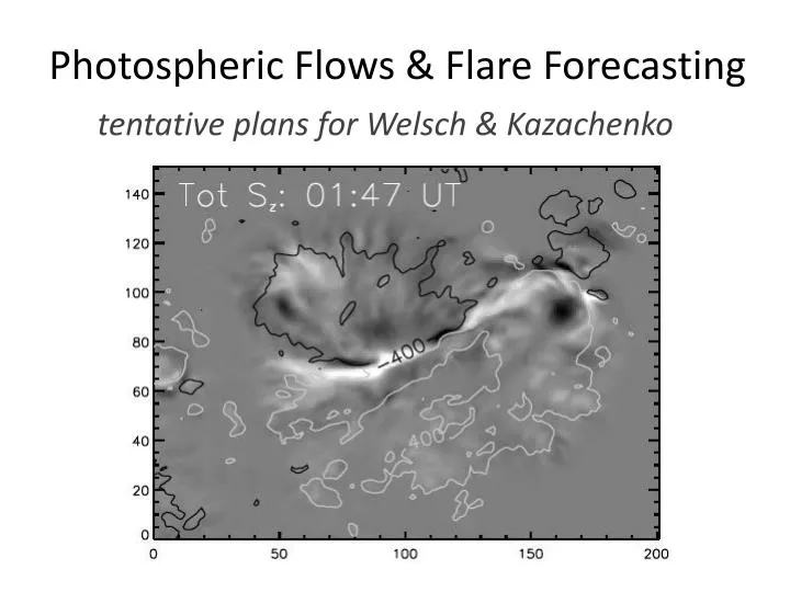
Photospheric Flows & Flare Forecasting tentative plans for Welsch & Kazachenko

Topics 0. Why do should photospheric electric or velocity fields Eor v matter for flares? • Previous work with BLOS • New opportunities with vector B

Aphotosphericelectric field E derived from magnetogram evolution can quantify aspects of evolution in Bcorona. • The fluxes of magnetic energy & helicityacross the magnetogram surface into the corona depend upon E: dU/dt = ∫ dA (E x B)z /4π dH/dt = 2 ∫ dA (E x A)z U and H probably play central roles in flares / CMEs. • Assuming Bph evolves ideally (e.g., Parker 1984), then photospheric flow and electric fields are related: cE = -(v x B)

The ideal assumption relates dBz/dt to v. • The magnetic induction equation’s z-component relates the flux transport velocity u to dBz/dt (Demoulin & Berger 2003): Bz/t = -c[  x E ]z= [  x (v x B) ]z = -  (u Bz) • Many tracking (“optical flow”) methods to estimate u have been developed, e.g., LCT (November & Simon 1988), FLCT (Fisher & Welsch 2008), DAVE (Schuck 2006).

The apparent motion of magnetic flux in magnetograms is the flux transport velocity, u. Démoulin & Berger (2003): In addition to horizontal flows, vertical velocities can lead to u ≠0. In this figure, vhor= 0, but vz ≠0, sou ≠ 0. uis not equivalent to v; rather,uvhor - (vz/Bz)Bhor • u is the apparent velocity (2 components) • vis the actual plasma velocity (3 components) (NB: non-ideal effects can also cause flux transport!) z z hor

We studied flows {u} from MDI magnetograms and flares from GOES for a few dozen active region (ARs). • NAR = 46 ARs from 1996-1998 were selected. • > 2500 MDI full-disk, 96-minute cadence, line-of-sight magnetograms were compiled • We estimated flows in these magnetograms using two separate tracking methods, FLCT and DAVE. • The GOES soft X-ray flare catalog was used to determine source ARs for flares at and above C1.0 level.

Magnetogram Data Handling • Pixels > 45o from disk center were not tracked. • To estimate the radial field, cosine corrections were used, BR = BLOS/cos(Θ). [dirty laundry!] • Mercator projections were used to conformally map the irregularly gridded BR(θ,φ) to a regularly gridded BR(x,y). • Corrections for scale distortion were applied.

Sample maps of FLCT and DAVE flows show them to be strongly correlated, but far from identical. When weighted by the estimated radial field |BR|, the FLCT-DAVE correlations of flow components were > 0.7.

Many parameters were studied…

Discriminant analysis can test the capability of one or more magnetic parameters to predict flares. 1) For one parameter, estimate distribution functions for the flaring (green) and nonflaring (black) populations for a time window t, in a “training dataset.” 2) Given an observed value x, predict a flare within the next t if: Pflare(x) > Pnon-flare(x) (vertical blue line) From Barnes and Leka 2008

Given two input variables, DA finds an optimal dividing line between the flaring and quiet populations. Blue circles are means of the flaring and non-flaring populations. The angle of the dividing line can indicate which variable discriminates most strongly. We paired field/ flow properties “head to head” to identify the strongest flare discriminators. (\ Standardized Strong-field PIL Flux R Standardized “proxy Poynting flux,” SR = Σ uBR2

We used discriminant analysis to pair field/ flow properties “head to head” to identify the strongest flare associations. For all time windows, regardless of whether FLCT or DAVE flows were used, DA consistently ranked Σu BR2among the two most powerful discriminators.

What’s the physics behind the SR-flare association? Yan Li (UC Berkeley / SSL) has suggested that: • SR is a proxy for the actual Poynting flux, • flares are more likely when the cumulative coronal energy is higher. From Li, Welsch, Lynch, Luhmann, & Fisher 2011

The “proxy Poynting flux” SR =Σu BR2 bears further study… With MDI, we found R and the proxy Poynting flux (PPF) to be most strongly associated with flares. Our sample size was small, so must redo this with larger N! Our results were empirical; we still need to understand the underlying processes. Also, it’ll be good to compare our parameter SR with others. For more details, see Welsch et al., ApJ v. 705 p. 821 (2009)

We have developed a way to use vector tB (not just tBz) to estimate E (or v). • Previous “component methods” derived vor Eh from the normal component of the ideal induction equation, Bz/t = -c[ hxEh ]z= [ x(vx B) ]z • But the vectorinduction equation can place additional constraints on E: B/t = -c(xE)= x(vx B), where I assume the ideal Ohm’s Law,*so v<--->E: E = -(vx B)/c==>E·B = 0 *One can instead use E = -(vx B)/c + R, if some model resistivity R is assumed. (I assume R might be a function of B or J or ??, but is not a function of E.)

The “PTD” method employs a poloidal-toroidal decomposition of B into two scalar potentials. ^ ^ ^ ^ tB = x (xtBz) +xtJztBz= h2(tB) 4πtJz/c= h2(tJ) h·(tBh) = h2(z(tB)) B =  x ( xB z) +xJz Bz = -h2B, 4πJz/c= h2J, h·Bh= h2(zB) Left: the full vector field B in AR 8210. Right: the part of Bh due only to Jz.

Faraday’s Law implies that PTD can be used to derive an electric field E from tB. ^ ^ “Uncurling” tB = -c(xE) gives EPTD = (hxtBz) +tJz Note: tB doesn’t constrain the “gauge” E-field -ψ! So: Etot = EPTD - ψ Since PTD uses only tB to derive E, (EPTD - ψ)·B = 0 can be solved to enforce Ohm’s Law (Etot·B = 0). (But applying Ohm’s Law still does not fully constrain Etot.)

PTD has two advantages over previous methods for estimating E (or v): • In addition to tBz, information from tJz is used in derivation of E. • No tracking is used to derive E, but tracking methods (ILCT, DAVE4VM) can provide extra info! For more about PTD, see Fisher et al. 2010, in ApJ 715 242

Doppler shifts and tranverse fields Btrs on LOS PILs can improve estimates of E. Will we get vLOS, Graham? Near a Polarity Inversion Line (PIL) of BLOS, B is purely transverse to vLOS We can thus measure a Doppler electric field EDopp= -(vLOS x Btrs)/c related to flux emergence at PILs. See Fisher et al. 2012, Sol. Phys. 277, 153 We can combine this info with the PTD B to improve our estimate of E

In tests with simulated MHD data, our reconstructed Poynting flux compared well with the true Sz. Qualitative and quantitative comparisons show good recovery of the simulation’s E-field and vertical Poyntingflux Sz.

We haven’t tested the Poynting flux from the PTD approach as a flare predictor, but hope it works! Also, it’ll be good to compare our parameter Sz with others.

Photospheric Flows & Flare Forecasting