Download
1 / 46
460 likes | 518 Views
Understand the Sun's magnetic cycle, convection zone dynamics, and impact on climate and space environment in this comprehensive study. Learn about magnetic field, solar activity, and dynamics of the Sun's internal structure.

E N D
Solar Photospheric Flowsand theSunspot Cycle David H. Hathaway NASA/Marshall Space Flight Center National Space Science and Technology Center 9 January 2009
Outline • Introduction • The Sun’s Magnetic Cycle • Convection Zone Dynamics • Magnetic Flux Transport Models • Modeling the Surface Flows • Conclusions
Introduction Why we study the solar cycle.
The Sunspot Cycle The Solar Activity Cycle is most easily seen in the number of sunspots and sunspot groups visible on the Sun. The average cycle is about 11 years long from sunspot number minimum to minimum. The amplitudes (average sunspot number at cycle maximum) of the sunspot cycle vary widely. The Sun shows periods of inactivity like the Maunder Minimum and periods of high activity like the last 50 years. The solar cycle has important societal impacts.
The Climate Connection Solar cycle related variations are evident in the terrestrial temperature record. Estimates of the variations in temperature at the Earth’s Surface (Mann et al. 1998, Moberg et al. 2005) show significant correlations with variations in the amplitude of the sunspot cycle. The total solar irradiance has varied by about 0.1% over each sunspot cycle since 1975. The UV irradiance varies by about 3-4%. The precise connections between solar variability and climate are uncertain.
Galactic Cosmic Ray Modulation The solar activity cycle modulates the radiation environment in the inner solar system. While the flux of Solar Energetic Particles (SEP) from solar flares and coronal mass rises and falls with the sunspot number, the flux of Galactic Cosmic Rays (GCR) is low when sunspot number is high.
Satellite Drag Credit: S.Solomon The solar activity cycle modulates the temperature and density of the thermosphere. Variations in the Sun’s UV and EUV irradiance over a solar cycle produce order of magnitude changes in the density at some spacecraft altitudes.
The Sun’s Magnetic Cycle A 160 year old mystery.
Magnetic Polarity- Joy’s Law Credit: Abbett, Fisher, & Fan (2001) Active regions are tilted with the leading spots closer to the equator than the following spots. This tilt increases with latitude. This is well modeled by the effect of the Coriolis force on magnetic flux tubes rising from deep inside the Sun.
Magnetic Polarity - Hale’s Law The magnetic polarity of the leading sunspots in active regions switches from one hemisphere to the other and from one cycle to the next.
Equatorward Drift Sunspots appear in bands on either side of the equator that drift toward the equator as each cycle progresses. Cycles overlap near the time of minimum. Each cycle is an individual outburst.
Polar Field Reversals The magnetic polarities of the Sun’s poles reverse from one cycle to the next at about the time of sunspot cycle maximum. The source of these reversals is the transport of following (higher latitude by Joy’s Law) polarity magnetic elements to the poles by a meridional flow.
Convection Zone Dynamics The fluid flow controls the magnetic field.
The Sun’s Internal Structure Energy is created in the Sun’s core by hydrogen burning and is carried outward by radiation (photons) through the core and radiative zone. The energy is carried outward by convective motions from a depth of about 200 Mm to the surface (the photosphere).
Measuring CZ Flows 1. Feature Tracking Measure the apparent motion of intensity (sunspots, granulation) or magnetic features. This gives both components of horizontal flow but depends upon availability of features (sunspots) and/or size of window for cross-correlations. Sunspots are known to have motions that do not reflect the actual surface flows.
Measuring CZ Flows 2. Doppler Measurements Measure the Doppler shift of photospheric spectral lines. This only gives the line-of-sight velocity but can provide data from the entire disc at rapid cadence.
Measuring CZ Flows 3. Helioseismic Measurements Measure the rotation of global oscillation modes (global helio-seismology) or differences in travel times for acoustic waves moving from point A to point B (local helioseismology). Gives horizontal flows as functions of latitude, longitude, and depth.
The Axisymmetric Flows All three methods give similar results – the rotation rate is faster at the equator and slower at the poles and the fluid flows from the equator to the poles at the surface.
Internal Rotation Profile Helioseismology gives the internal rotation profile. There are shear layers at the top and bottom of the convection zone. The latitudinal variation seen at the surface vanishes at the CZ base.
Internal Meridional Flow The poleward meridional flow persists to depths of at least 20 Mm. A slow return flow below 0.8 R is suggested by mass flow constraints.
Non-Axisymmetric Flows Supergranules Hart (1954) Granules Dawes (1864)
Granules • Cellular flow pattern • Characteristic Width ~ 1 Mm • Characteristic Lifetime ~ 10m • Typical flow velocities ~ 3 km/s • Magnetic elements form in the downdrafts at the corners • Flow velocities can become supersonic ( > 7 km/s) and generate acoustic waves • Size is characteristic of pressure scale height at photosphere • Well modeled in radiative-MHD simulations
Supergranules • Cellular flow pattern • Characteristic Width ~ 30 Mm • Characteristic Lifetime ~ 1d • Typical flow velocities ~ 300 m/s • The magnetic network forms at their boundaries • They drive the surface shear • NOT well modeled in any simulations • Rotation Rate mysteries • Faster for longer time lags • Faster for bigger cells • Faster than the internal rotation? • Open Question: What determines their characteristic size?
Giant Cells Giant cells – convection cells that span the CZ – were proposed in the 1950s and 1960s. They appear in numerical simulations. Their north-south alignments are critical to driving the differential rotation. Their existence is suggested by observations but definitive characteristics have not been determined.
Mesogranules Mesogranules – cells intermediate in size between granules and supergranules – were proposed in the 1981 by November, Toomre, and Gebbie. They filtered out the granules and then the supergranules and found a residual pattern with typical sizes of 10 Mm and lifetimes of hours.
Basic Dynamo Processes Two basic dynamo processes are common to most models – shearing of poloidal field lines by differential rotation and lifting and twisting of toroidal field lines. The emerging field must still be transported poleward by diffusion and/or meridional flow.
Dikpati & Charbonneau Dynamo In/CCW Out/CW This is a 2D kinematic dynamo which uses the observed internal differential rotation, a realistic meridional circulation, a low diffusivity, and a parameterized α-effect. It produces a reversing magnetic field configuration with a 22-year period and an equator-ward propagation of active zones. Strong Meridional flow gives strong polar fields. This model is used in predicting Cycle 24.
Surface Flux Transport Surface flux transport models take emerging active regions as input and transport the magnetic flux by differential rotation, meridional flow, and diffusion. Strong Meridional flow gives weak polar fields. This model is use to give historical field estimates.
Spherical Harmonic Analysis Years ago I developed an analysis technique based on spherical harmonics. The axisymmetric flows are determined and extracted. The nonaxisymmetric flows are projected onto spherical harmonics.
Data Simulations • Calculate vector velocities using input spectrum of complex spectral coefficients, R, S, and T (Chandrasekhar, 1961). • Project velocities into the line-of-sight, integrate over pixels, add noise, and blur with MDI MTF to get the observed signal
Spectral Comparison Observed kinetic energy per wavenumber matches. The input spectrum has two Lorentzian-shaped components: supergranules and granules.
Evolving the Flow Pattern • The velocity pattern is evolved using the advection equation • where, for example, • plus random changes in the phases of the complex coefficients so that the accumulated changes are of order 1 for a turnover time
Rotation Profiles fromCross-Correlation Studies Near the equator faster rotation rates are obtained for larger separations in time. This was previous noted by Duvall (1980) and by Snodgrass & Ulrich (1990).
Rotation Profile Comparisons They match at virtually all latitudes and time differences.
Lifetime Comparisons The correlation match extremely well for separations of 8h and 16h. The correlations are a bit too high for the shortest separations – suggesting faster evolution or more noise.
Rotation Rate vs. Wavenumber Beck & Schou (2000) Figure 4 10-day Simulation Results The increase in rotation rate at small wavenumbers – to rotation rates greater than the maximum measured by helioseismology in the surface shear layer – suggested a wave-like nature for supergranules. The rotation rate we use DOES NOT exceed the maximum. The faster rates are an illusion due to the line-of-sight projection of the Doppler observations.
Wave-Like Properties? Schou (2003) found evidence for prograde and retrograde moving components after adjusting for projection effects, applying weighting and apodizing functions, and tracking at an appropriate rotation rate. MDI – 60d @ 1/60m SIM – 10d @ 1/15m
Key Points • We simulate photospheric velocity fields that accurately reproduce the MDI observations. They show: • Only two cellular flows are implicated: granules and supergranules. • The cellular flows need not rotate faster than the layers they are embedded in. • The simulated velocity fields are useful for other studies, e.g. magnetic element diffusion.
Magnetic Element Diffusion The simulated flows can be used to advect passive elements to determine the characteristics of diffusion.
Meridional Flow Variations 2000 1996 2008 2003 I have started measuring the meridional flow using feature tracking on weak field magnetic elements and find variations over the course of cycle 23 (min. in 1996, max. in 2000, min. in 2008).
Conclusions • There are two components to the surface cellular flows - supergranules and granules. • Supergranules do not actually rotate more rapidly than the peak rotation rate in the surface shear layer. • The simulated flow fields can now be used to study the magnetic field diffusion characteristics. • Variations in the flows over time can be used to distinguish between different flux transport models.