Mastering R Graphics: Creating, Customizing, and Enhancing Charts
This module focuses on harnessing R's powerful graphical capabilities to create stunning charts. Learn how to construct a graphic script, utilize R's diverse graphics packages (like ggplot2 and lattice), and gain precise control over graphics parameters. You'll explore different areas of charts, including plot, figure margin, and outer margin, while mastering both high-level and low-level graphic functions. Through hands-on examples, you'll gain proficiency in adding text, lines, and customizations to bring your data visualizations to life.

Mastering R Graphics: Creating, Customizing, and Enhancing Charts
E N D
Presentation Transcript
Module 4R Charts Do Learn See & Hear Read PowerPoint must be in View Show Mode to See videos and hyperlinks R Charts
Module 4 R Graphics Menu • Making a Graphic Script • Working with plot() Function • Adding Text to a Chart • Adding Lines to Chart • Extra R Scripts R Charts
Menu Making a Graphic Script Click video image to start video R Charts
Menu Making a Graphic Script • R’s Graphic Packages • R’s 3 Distinct Chart Areas • Script Components • High level functions • Graphic parameters • Low level Functions R Charts
Menu R’s Graphics Packages • R has several graphics subsystems: • Graphics – traditional graphics • Grid package (low level functions) • Lattice package • ggplot2 package • This module shows the traditional - base graphics system R Charts
R’s 3 Chart Areas: Plot Area – within axes Figure Margin Area – for axis labels and tick mark labels Outer Margin Area R gives User precise control over content, format of all 3 Areas High Level Graphic Functions Graphic Parameters Low Level Graphic Functions Menu R’s 3 Distinct Chart Areas R Charts
# R Script to produce scatter chart x_data <- ...y_data <-…par( ) # Graphic parametersplot( ) # High level plot functiontext( ) # Low level function Menu Making a Graphic Scriptwith R’s Graphic Package High Level Graphic Function Call Use GP defaults or adj GP w/ argument Low Level Graphic Function Call Use GP defaults or adj GP w/ argument Graphic Parameters 70 GPs defaults set adjust w/ par() par(oma=c(2,2,2,2)); par(mar=c(3,3,1,1))plot(x_data, y_data, main = “My Chart Title“, type = "b",xlim = c(0,11), ylim = c(0,11), xlab ="X", ylab = "Y“, pch=16, col = "red", bty = "n", xaxs="i", yaxs = "i", las=1) text(2,7, “my note”,col = “blue” ) R Charts
Menu High Level Graphic Functions Produce complete chart This module focuses on plot() function low level functions, graphic parameters. Module 5 covers box, dot, histogram and strip charts R Charts
Menu Low Level Plot FunctionsAdd graphic content to current plot R Charts
R has 70 Graphic Parameters (GP) Each GP has: name: col = value: “red” Default Values Set At start of R session To Get par() values par() lists all 70 with current value par(“GP_name”) gives current value for specific GP User can change GP value: Global: par(“col” = “red”) Local: plot(x,y,col=“red”) Menu Graphic ParametersGP > par(“col”) [1] “black” R Charts
Menu Essential Graphical Parameters* These parameters must be set with call to par(). R Charts
Menu pch = Plot Characters Graphic Parameter • R has 25 plotting characters • pch = specifies plot character • Characters 19 – 20 can be filled with selected color • 19 – Solid circle • 20 – Bullet circle • Characters 21: 25 can have selected fill and border colors • bg = Controls Border color • col= Controls fill R Charts
Menu lty= Line Type Graphic Parameter • R has 6 line types • lty = specifies the line type • lty= can be specified as integer or character string: • 0 – “blank” • 1 – “solid” • 2 – “dashed” • 3 – “dotted” • 4 – “dotdash” • 5 – “longdash” • 6 – “twodash” R Charts
Menu Assignment 4-1Getting Familiar with par() • Print out par documentation ?par • Get Current Values for all par() • Get current par(“bty”) value R Charts
Menu Working with plot() Function Click video image to start video R Charts
Menu plot() Function Arguments plot(x,y, type=“?”, main’”??”, sub = “??“, xlab=“??”, ylab =“??”, ann =?, axes = ?, xlim = c(x1,x2), ylim = c(y1,y2)) or plot(y ~ x, data = “??”, type=“?”, main’”??”, sub = “??“, xlab=“??”, ylab =“??”, ann =?, axes = ?, xlim = c(x1,x2), ylim = c(y1,y2)) R Charts
# R script to demonstrate default plot() ## Ex_Scr_4_1_default_plot.R ################### ##Script to produce default XY plot() ## STEP 1: SETUP - Source File rm(list=ls()); par(oma=c(2,1,0,1)) script = "C:/Learn_R/Mod_4_R_Charts/Ex_Scr_4_1_default_plot.R" ## STEP 2: READ DATA y_data <- c(0,1,2,3,4,5,6,7,8,9,10,9,8,7,6,5,4,3,2,1,0) x_data <- seq(0:20) ## STEP 3: MANIPULATE DATA ## STEP 4: PRODUCE CHART - REPORT plot(x_data,y_data, main = "plot() Defaults ") ## Outer Margin annotation my_date <- format(Sys.time(), "%m/%d/%y") mtext(script, side = 1, line = .75, cex=0.7, outer = T, adj = 0) mtext(my_date, side = 1, line =.75, cex = 0.7, outer = T, adj = 1) Menu plot() Function Defaults • Potential plot() Default Improvements • Line – symbol style • X & Y axis do not meet @ 0 • Remove box around plot • Adjust Y axis label orientation • Improve X & Y axis labels R Charts
plot(x_data,y_data, main = "plot() Default Improvements", type = "b",col = "red", bty = "n", xaxs="i", yaxs = "i", las=1, xlim = c(0,25), ylim = c(0,12), xlab = "X", ylab = "Y" ) plot(x_data,y_data, main = "plot() Defaults" ) Menu Improving plot() Function Defaultswith Additional plot() arguments & graphical parameters R Charts
Users can specify colors by name; R has 657 colors “red” “blue” “darkgreen” To get list of R colors: >colors() col = most common way to specify color for lines, points, text Alternatives: rgb() and hsv() Color Conversions: col2rgb() convertColor() Menu Working With R Colors R Charts
Menu plot() type argument type=?, • "p" for points • "b" for both • "o" for both ‘overplotted’ • "l" for lines • "c" for the lines part alone of "b" • "h" for high-density vertical lines • "s" for h/v stair steps • "S" for v/h stair steps • "n" for no plotting R Charts
Menu Example Scatter plot ## Ex_Scr_4_3_xy_plot.R ################### ##Script to produce scatter plot ## STEP 1: SETUP - Source File rm(list=ls()); par(oma=c(2,1,0,1)) script <- "C:/Learn_R/Mod_4_R_Charts/Ex_Scr_4_3_xy_plot.R" ## STEP 2: READ DATA x_data <- seq(0,10*pi,0.1*pi) y_data <- sin(x_data) plot(x_data,y_data,type = "l") ## Outer margin annotation my_date <- format(Sys.time(), "%m/%d/%y") mtext(script, side = 1, line = .75, cex=0.7, outer = T, adj = 0) mtext(date(), side = 1, line =.75, cex = 0.7, outer = T, adj = 1) R Charts
Start R Session In R Console, Open Script: “C:/Learn_R/Mod_4_R_Script/Ex_Scr_4_3_xy_plot.R” Save as: “C:/Learn_R/Mod_4_R_Script/Practice_4_1_xy_plot.R” Make these changes par() settings: par(ps = 10) par(las = 1) plot() formatting: type = “b” pch = 16 col = “blue” xlab = “X”; ylab= “sin(X)” main = “xy Plot of sin() Formula” xlim = c(0, 15) ylim = c(-2, 2) Menu Assignment 4-2xy plot () Expected Result R Charts
Menu Assignment 4-2xy plot () ## Practice_4_1_xy_plot.R ################### ##Script to produce scatter plot ## STEP 1: SETUP - Source File rm(list=ls()); par(oma=c(1.75,1,0,1)); par(las=1); par(ps=10) script <- "C:/Learn_R/Mod_4_R_Charts/Practice_4_1_xy_plot.R" ## STEP 2: READ DATA x_data <- seq(0,10*pi,0.1*pi) y_data <- sin(x_data) plot(x_data,y_data,type = "b",pch = 16, col = "blue", xlab ="X", ylab = "sin(X)", main = "xy Plot of sin() Function", xlim = c(0,15), ylim = c(-2,2)) ## Outer margin annotation my_date <- format(Sys.time(), "%m/%d/%y") mtext(script, side = 1, line = .5, cex=0.7, outer = T, adj = 0) mtext(date(), side = 1, line =.5, cex = 0.7, outer = T, adj = 1) Assignment 4-2 Script R Charts
Menu Assignment 4-3Make Step Chart and Scatter Plot Interactively Edit Your Practice_4_1_xy_plot.R Script to make these charts type = ‘s” type = ‘p” R Charts
Menu Working With Text Click video image to start video Text is Critical for chart interpretation R Charts
Text Additions: main= argument to add chart title in figure margin at top sub= argument to add subtitle below X axis text() – low level function to add text in plot area mtext() – low level function to add text in margin and outer areas Size: par(ps=10) Magnification: cex = 0.85 Color: col=“red” (657 color choices) font= 1-4 (regular, bold, italic, bold italic) family= (“sans”, “serif”, “mono”) Alignment: adj = 0,.5,1(left,center, right) Rotation: srt= Menu Working With Text Text is Critical for chart interpretation R Charts
text( x, y, “note”, pos =0 , cex = 1, col = “red”, srt = 45) x,y – plot area coordinates where text should be placed “note” – text to be added to plot pos – position of text with respect to x, y coordinates. Default is centered on point. cex - font magnification factor col - color srt – text rotation - degrees User can construct multi-line text strings by using \n to designate new line Note <- “This is an example \n of a multi-line note ” Menu Adding text string in Plot Areatext () Function \n for Multi-line Text \”to add quote marks to text string • Text strings designated by “ “ marks • User can embed quote marks within text string by using \” to have R not treat mark as begin/end of text string • Note <- “This is an example of using \”quote marks\” within text string” R Charts
Menu Simple Plot – No Annotation #################### Example R Script: ############### ## Ex_Scr_4_4_simple_plot.R ######################## ##Script to read data file, simple plot ## STEP 1: SETUP - Source File rm(list=ls()); oldpar<- par(no.readonly=T); ;par(las=1) link <- "C:\\Learn_R\\Mod_4_R_Charts\\Data_4_1_GISS_1980_By_year.txt.txt" ## STEP 2: READ DATA my_data <- read.table(link, skip =0, sep = ",", dec=".", row.names = NULL , header = F, colClasses = c("numeric","numeric"), comment.char = "#", na.strings = c( "","*", "-",-99.9, -999.9 ), col.names = c( "yr", "anom") ) attach(my_data) ## STEP 3: MANIPULATE DATA ## STEP 4: PRODUCE PLOT - REPORT plot(yr, anom, type = "l", col = "red") ## Outer margin annotation my_date <- format(Sys.time(), "%m/%d/%y") mtext(script, side = 1, line = .5, cex=0.7, outer = T, adj = 0) mtext(my_date, side = 1, line =.5, cex = 0.7, outer = T, adj = 1) ## STEP 5: CLOSE par(oldpar) detach(my_data) R Charts
Menu Simple Plot –with Annotation #################### Example R Script: ############### ## Ex_Scr_4_5_simple_plot_w_annotation.R ######################## ##Script to read data file, simple plot ## STEP 1: SETUP - Source File rm(list=ls()) script<- "C:\\Learn_R\\Mod_4_R_Charts\\Ex_Scr_4_5_simple_plot_w_annotation.R" oldpar<- par(no.readonly=T) par(oma=c(2,2,1,2)); par(las=1); par(mar=c(5,4,2,1)) link <- "C:\\Learn_R\\Mod_4_R_Charts\\Data_4_1_GISS_1980_By_year.txt.txt" ## STEP 2: READ DATA my_data <- read.table(link, skip =0, sep = ",", dec=".", row.names = NULL , header = F, colClasses = c("numeric","numeric"), comment.char = "#", na.strings = c( "","*", "-",-99.9, -999.9 ), col.names = c( "yr", "anom") ) attach(my_data) ## STEP 3: MANIPULATE DATA m_title <- "GISS Temperature Anomaly - C (1980-2008)" sub_title <- "Source: http://data.giss.nasa.gov/gistemp/" note <- "Baseline 1951-1980" ## STEP 4: PRODUCE PLOT - REPORT plot(yr, anom, type = "l", col = "red", main = m_title, sub = sub_title, ylab = " Temperature Anomaly - C", xlab = "", cex.axis = 0.75, cex.lab=0.8, cex.main = .8, cex.sub = 0.6) text(1985,0.65, note, cex=0.6 ) my_date <- format(Sys.time(),"%m/%d/%y") mtext(script, side=1, line = .5, outer = T, adj = 0, cex = 0.65) mtext(my_date, side = 1, line = 0.5, outer = T, adj = 1, cex = 0.7) ## STEP 5: CLOSE par(oldpar); detach(my_data) R Charts
font= font type for plot text =1 Standard =2 Bold =3 Italic =4 Bold and italic Use for other figure text font.axis; font.lab font.main; font.sub family = controls font family = “sans” = “serif” = “mono” Menu text()font & family R Charts
paste(arg1, arg2, arg3, sep= “ ”) arg1 – text string or variable to be concatenated with other arguments sep = “ ” - separator to add between arguments. Space good for text. Variable data and text strings can be concatenated into a single string that can then be added to plot with text() Example: # build text string with paste() my_date <- paste(“today is “, date()) # add text string to plot text(x, y, my_date, col = “red”) Menu paste() Functionconcatenates arguments into a single string R Charts
mtext( “note”, side = , line = , outer = F, adj = 0, cex = 1, col = “red”) “note” – text to be added to margin area side – side of plot to place text(1= bottom, 2= left, 3= top, 4=right) line – line of margin to place text, starting at 0, counting outwards outer – use outer area (T or F) adj – text alignment, 0 = left, 0.5= center, 1 = right cex - font adjustment factor col - color Axis Numbering Convention 3 Axis Sides 2 4 1 Menu Adding Text within Margin Area R Charts
Menu How I’ve Been Adding Margin Text to Each Mod 4 Plot • 3 Steps to Create Margin Annotation: • Set Outer Margin Areas • par(oma=c(2,2,0,1)) • Establish script name vector • script<- "C:\\Learn_R\\Mod_4_R_Charts\\Ex__plot_.R" • Develop Margin Text w/date & script name • ## Outer margin annotation • my_date <- format(Sys.time(), "%m/%d/%y") • mtext(script, side = 1, line = .5, cex=0.7, outer = T, adj = 0) • mtext(my_date, side = 1, line =.5, cex = 0.7, outer = T, adj = 1) R Charts
Start R Session In R Console, Open Script: “C:/Learn_R/Mod_4_R_Script/Ex_Scr_4_3_simple_plot.R” Save as: “C:/Learn_R/Mod_4_R_Script/Practice_4_2_my_simple.R” You’ve seen me do it Make the Full Annotation on your own Menu Assignment 4-4Annotate Simple Chart Yourself R Charts
Menu Adding Lines in Plot Area Click video image to start video R Charts
Menu Adding Lines in Plot Area #################### Example R Script: ############### ## Ex_Scr_4_6_add_lines_to_plot.R ######################## ##Script to read data file, simple plot no annotation ## STEP 1: SETUP - Source File rm(list=ls()) script<- "C:/Learn_R/Mod_4_R_Charts/Ex_Scr_4_6_add_lines_to_plot.R" oldpar<- par(no.readonly=T) ; par(las=1) par(ps=10); par(oma=c(2,2,1,2)) ## STEP 2: READ DATA x <- 0:100; y <- x^2 x_pts <- c(15, 35, 35, 15, 15); y_pts <- c(8300, 8300, 6500, 6500,8300) # STEP 3: MANIPULATE DATA # STEP 4: PRODUCE CHART - REPORT plot(x,y, type = "n“ , main="Add Lines, Points, Arrows Examples") points(x, y,col = "black", lty=1, type = "l") grid(col="lightgrey", lty=1) abline(h=2500, col="red") abline(v=50, col = "blue") arrows(65,8400, 85,8400, code=3, col="orange", length = 0.1) lines(x_pts, y_pts, lty=1, col = "green") points(x_pts,y_pts, type = "p",col ="red",pch=19) my_date <- format(Sys.time(),"%m/%d/%y") mtext(script, side=1, line = .5, outer = T, adj = 0, cex = 0.65) mtext(my_date, side = 1, line = 0.5, outer = T, adj = 1, cex = 0.7) ## STEP 5: CLOSE par(oldpar) detach(my_data) R Charts
Start R Session In R Console, Open Script: “C:/Learn_R/Mod_4_R_Script/Ex_Scr_4_6_add_lines_to_plot.R” Save as: “C:/Learn_R/Mod_4_R_Script/Practice_4_3_add_lines_to_plot.R” You’ve seen me work with it Changes each element to see what happens, get comfortable with forms of lines Menu Assignment 4-5Working with grid(), points(), abline(), arrows() & lines() Printout & Read R Documentation for lines ? grid() ? points() ? lines() ? abline() ? arrows() R Charts
Menu Extra Scripts Click video image to start video R Charts
Plot Box & Axis Options Box type bty=“n” bty=“o” Axes axes = T or F Axis Offset: xaxs= “i” or “r” yaxs = “i” or “r” Axis 3 & 4 tick marks Axis(n, ..tick=T) Menu Plot Box and Axis Styles R Charts