RF Engineering Introduction
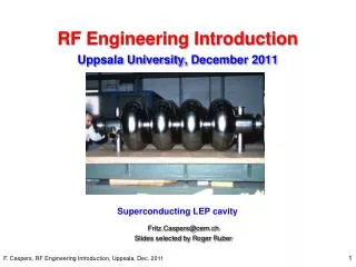
RF Engineering Introduction. Uppsala University, December 2011. Superconducting LEP cavity. Fritz.Caspers@cern.ch Slides selected by Roger Ruber. RF Tutorial Contents. Part I Basics Cavity structures Equivalent circuit Characterisation in time and in frequency domain

RF Engineering Introduction
E N D
Presentation Transcript
RF Engineering Introduction Uppsala University,December 2011 Superconducting LEP cavity Fritz.Caspers@cern.ch Slides selected by Roger Ruber
RF Tutorial Contents Part I • Basics • Cavity structures • Equivalent circuit • Characterisation in time and in frequency domain • Beam-cavity interaction Part II • Diagnostics using RF instrumentation • Wall current monitor • Button pick-up • Cavity type pick-up • Travelling wave structures • Possibilities and limitations of Schottky diagnostics Contents
From L and C to a cavity If you open the beam pipe then both ends are at the same potential Creates E-field for accelerating the particles put a cavity in there Ez Beam Short circuit, thus no scalar potential difference Can the short-circuit be avoided? Answer: No - but it doesn’t bother us at high frequencies. Capacitor at high frequencies, The Feynman Lectures on Physics Basics
Maxwell’s equations (1) scalar vs. vector potential: path of integration makes a difference Basics
Maxwell’s equations (2) ·D = with the charge density r ·B = 0 There are no magnetic charges Basics
Displacement and conduction currents in a simple capacitor end plates = sides planes of a pillbox cavity for vacuum and approximately for air:m = m0 = 4p*10-7 = 1.2566 * 10-6 Vs/(Am)e = e0 = 8.854*10-12 As/(Vm) E E The conduction current continues as displacement current over the capacitor gap Displacement current in dielectric: Conduction current in conductor: with the electric flux FD and the charge Q. Basics
General Solution for a Rectangular (brick-type) Cavity When describing field components in a Cartesian coordinates system (assuming a homogeneous and isotropic material in a space charge free volume) with harmonic functions (angular frequency ) then each Cartesian component needs to fulfill Laplace's equation: As a general solution we can use the product ansatz for From this one obtains the general solution for ( may be a vector potential or field) with the separation condition standing waves travelling waves see also: G. Dome, RF Theory Proceeding Oxford CAS, April 91 CERN Yellow Report 92-03, Vol. I Basics
General Solution in Cylindrical Coordinates As a general solution we can use the product ansatz for From this one obtains the general solution for ( may be a vector potential or field) and the functions Here the separation condition is standing waves travelling waves Hint: the index m indicating the order of the Bessel and Neumann function shows up again in the argument of the sine and cosine for the azimuthal dependency. Basics
Bessel Functions (1) A nice example of the derivation of a Bessel function is the solution of the cylinder problem of the capacitor given in the Feynman reference (Bessel function via a series expansion). Comment: For the generalized solution of cylinder symmetrical boundary value problems (e.g. higher order modes on a coaxial resonator) Neumann functions are required. Standing wave patterns are described by Bessel- and Neumann functions respectively, radially travelling waves in terms of Hankel functions. Hint: Sometimes a Bessel function is called Bessel function of first kind, a Neumann function is Bessel function of second kind, and a Hankel function=Bessel function of third kind. J0 the term “root” stands for zero-crossing J1 J2 first root of the Bessel function of 0th order second root of the Bessel function of 1st order Basics
Bessel Functions (2) Some practical numerical values: See: http://mathworld.wolfram.com/BesselFunctionZeros.html Basics
Neumann Functions N0 N1 N2 Neumann functions are often also denoted as Ym(r). Basics
Electromagnetic waves E field of the fundamental TE10 mode • Propagation of electromagnetic waves inside empty metallic channels is possible: there exist solutions of Maxwell’s equations describing waves • These waves are called waveguide modes • There exist two types of waves, • Transverse electric (TE) modes: the electric field has only transverse components • Transverse magnetic (TM) modes: the magnetic field has only transverse components • Propagate at above a characteristic cut-off frequency In a rectangular waveguide, the first mode that can propagate is the TE10 mode. The condition for propagation is that half of a wavelength can “fit” into the cross-section => cut-off wavelengthc = 2a The modes are named according to the number of field maxima they have along each dimension. The E field of the TE10 mode for instance has 1 maximum along x and 0 maxima along the y axis. For circular waveguides, the maxima are counted in the radial and azimuthal direction Basics
Mode Indices in Resonators (1) TE101 =H101 E For a structure in rectangular coordinatesthe mode indices simply indicate the number of half waves (standing waves) along the respective axis. Here we have one maximum along the x-axis, no maximum in vertical dimension (y-axis), and one maximum along the z-axis. TE101corresponds to TExyz Basics
Mode Indices in Resonators (2) TM010 = E010 For a structure in cylindrical coordinates: The first index is the order of the Bessel function or in general cylindrical function. The second index indicates “the root” of the cylindrical function which is the number of zero-crossings. The third index is the number of half waves (maxima) along the z-axis. Hint: In an empty pillbox there will be no Neumann function as it has a pole in the center (conservation of energy). However we need Bessel and Neumann functions for higher order modes of coaxial structures. Ez Ez -B The number m of maxima along the azimuth is coupled to the order of the Bessel function (see slide on theory). Basics
Fields in a pillbox cavity Cavity height: hcavity radius: aTM010 mode resonance = E010 mode resonance for TM010 resonance frequency independent of h!!!In the cylindrical geometry the E and H fields are proportional to Bessel functions for the radial dependency. Ez Ez a -B h Capacitor at high frequencies, The Feynman Lectures on Physics Cavity structures
Common cavity geometries (1) Square prism H101 or TE101 b E c a Comment: For a brick-shaped cavity (the structure is described in Cartesian coordinates) the E and H fields would be described by sine and cosine distributions. The mode indices indicate the number of half waves along the x-,y-, and z-axis, respectively. this simplifies in the case a=c: Cavity structures
Common cavity geometries (2) Circular cylinder: E010, = TM010 a E h B 1 for not too big ratios of h/a Note: h denotes the full height of the cavity In some cases and also in certain numerical codes, h stands for the half height 1: formula uses Linac definition and includes time transit factor Cavity structures
R/Q for cavities see lecture: RF cavities, E. Jensen, Varna CAS 2010 (First zero of the Bessel function of 0th order) The full formula for calculating the R/Q value of a cavity is with This leads to The sinus can be approximated by sinx = x (for small values of x) leading to
Common cavity geometries (3) Circular cylinder: H011 H111 Cavity structures
Common cavity geometries (4) Coaxial TEM b a short E h Coaxial line with minimum loss slide TEM transmission lines (3) short Taken from S. Saad et.al.,Microwave Engineers‘ Handbook, Volume I, p.180 Cavity structures
Common cavity geometries (5) Sphere Sphere with cones E 2a “Nose cone cavity” “Energy storage in LEP” the tips of the cone don’t touch a spherical “/4-resonator” Cavity structures
Mode chart of a brick-shaped cavity The resonant wavelength of the Hmnp resonance calculates as Reprinted from Meinke, H. and Gundlach, F. W.,Taschenbuch der Hochfrequenztechnik,S.471Erste Auflage, Springer-Verlag, Berlin (1968) and Techniques of Microwave Measurements by Carol G. Montgomery, 1st ed., 1947; by permission, McGraw-Hill Book Co., N. Y. for a Emn or a Hmn wave with p half waves along the c-direction. Cavity structures
Mode chart of a Pillbox cavity – Version 1 Cylindrical cavity with radius a, height = h and resonant wavelength l0.H stands for TE and E for TM modes. Reprinted from Meinke, H. and Gundlach, F. W.,Taschenbuch der Hochfrequenztechnik,S.471Erste Auflage, Springer-Verlag, Berlin (1968) and Techniques of Microwave Measurements by Carol G. Montgomery, 1st ed., 1947; by permission, McGraw-Hill Book Co., N. Y. Example: E010: l02.6a H111: h2aH112: h4a 2a Cavity structures
Mode chart of a Pillbox cavity – Version 2 H212 2.5 2 1.5 1 0.5 H112 E012 H011E111 H012E112 Cylindrical cavity with radius a, height = h and resonant wavelength l0.H stands for TE and E for TM modes. H211 E110 E011 Reprinted from Meinke, H. and Gundlach, F. W.,Taschenbuch der Hochfrequenztechnik,S.471Erste Auflage, Springer-Verlag, Berlin (1968) and Techniques of Microwave Measurements by Carol G. Montgomery, 1st ed., 1947; by permission, McGraw-Hill Book Co., N. Y. (2a/0)2 H111 Example: E010: (2a/l0)20.6 l0 2.6a H111: h2aH112: h4a E010 1 2 3 4 (2a/h)2 Cavity structures
Skin-effect and scaling laws for copper Skin-effect graph, plot for copper Reprinted from Meinke, H. and Gundlach, F. W.,Taschenbuch der Hochfrequenztechnik,Dritte Auflage, Springer-Verlag, Berlin (1968) and Techniques of Microwave Measurements by Carol G. Montgomery, 1st ed., 1947; by permission, McGraw-Hill Book Co., N. Y. Examples: Cavity structures
Equivalent circuit (1) The generator may deliver power to Rp and to the beam, but also the beam can deliver power to Rp and Rg! Beam Generator The beam is usually considered as a current source with infinite source impedance. Lossless resonator We have Resonance condition, when Resonance frequency: Equivalent circuit
Equivalent circuit (2) Characteristic impedance “R upon Q” Stored energy at resonance Dissipated power Q-factor Shunt impedance (circuit definition) Tuning sensitivity Coupling parameter (shunt impedance over generator or feeder impedance Z) (R/Q) is independent of Q and a pure geometry factor for any cavity or resonator! This formula assumes a HOMOGENEOUS field in the capacitor ! W ... stored energy P ... dissipated power Equivalent circuit
The Quality Factor (1) • The quality (Q) factor of a resonant circuit is defined as the ratio of the stored energy W over the energy dissipated P in one cycle. • The Q factor can be given as • Q0: Unloaded Q factor of the unperturbed system, e.g. a closed cavity • QL: Loaded Q factor with measurement circuits etc connected • Qext: External Q factor of the measurement circuits etc • These Q factors are related by Equivalent circuit
The Quality Factor (2) Q as defined in a Circuit Theory Textbook: Q as defined in a Field Theory Textbook: Q as defined in an optoelectronics Textbook: Reprinted from Madhu S. Gupta, Educator‘s Corner, IEEE MicroWave Magazine,Volume 11, Number 1, p. 48-59, February 2010. See also: G. Dome, CAS (CERN Accelerator School), Oxford, June 1992 Equivalent circuit
Transients on an RC-Element (1) I(t) V(t) Decay ~ e-t/ A voltage source would not work here! Explain why. Build up ~(1-e-t/) 63% of maximum 37% of maximum Behaviour in time and in frequency domain
Transients on an RC-Element (2) Behaviour in time and in frequency domain
Response of a tuned cavity to sinusoidal drive current (1) Drive current I In the first moment, the cavity acts like a capacitor, as seen from the generator (compare equivalent circuit). The RF is therefore short-circuitedIn the stationary regime, the inductive (wL) and capacitive reactances (1/(wC)) cancel (operation at resonance frequency!). All the power goes into the shunt impedance R => no more power reflected, at least for a matched generator... Cavity response U Behaviour in time and in frequency domain
Measured time domain response of a cavity Cavity E field (red trace) and electron probe signal (green trace) with and without multipacting. 200 μs RF burst duration. see: O. Heid, T Hughes, COMPACT SOLID STATE DIRECT DRIVE RF LINAC EXPERIMENTAL PROGRAM, IPAC Kyoto, 2010
Numerically calculated response of a cavity in the time domain see: I. Awai, Y. Zhang, T. Ishida, Unified calculation of microwave resonator parameters, IEEE 2007
Response of a tuned cavity to sinusoidal drive current (2) V... envelope amplitudeC... cavity capacitanceI... drive currentZ... cavity impedanceR... real part of cavity impedance Differential equation of the envelope (shown without derivation): are complex quantities, evaluated at the stimulus (drive) frequency.For a tuned cavity all quantities become real. In particular Z = R, therefore This value refers to the 1/e decay of the field in the cavity. Sometimes one finds w referring to the energy with 2w= . The voltage (or current) decreases to 1/e of the initial value within the time t. see also: H. Klein, Basic concepts I Proceeding Oxford CAS, April 91 CERN Yellow Report 92-03, Vol. I "Q over p periods" Behaviour in time and in frequency domain
Beam-cavity interaction (1) Cavity response in time domain c(t) from one very short bunch Bunched beamb(t) with bunch length tb, bunch spacing T and beam current I0 step height DU = q/Cremnant voltagefrom previous bunches Resulting response for bunched beam obtained by convolution of the bunch sequence with the cavity response r(t) = b(t) Äc(t)Condition that the induced signals in the cavity add up:cavity resonant frequency fres must be an integer multiple of bunch frequency 1/T Beam-cavity interaction
Beam-cavity interaction (2) For a quantitative evaluation the worst case is considered with the induced signals adding up in phase. Two approaches: Equilibrium condition: Voltage drop between two bunch passages compensated by newly induced voltage Summing up individual stimuli Beam-cavity interaction
Beam-cavity interaction in Frequency domain Frequency domain beam spectrum B(f)cavity response C(f)Resulting spectrum obtained by multiplicationR(f) = B(f) * C(f) We see strong central line with two sidebands. This is AM modulation. Where do you find this AM modulation in the time domain? Beam-cavity interaction
Typical parameters for different cavity technologies Beam-cavity interaction
Electromagnetic scaling laws A cavity of a given geometry can be scaled using three rules: The ratio of any cavity dimension to l is constant. To put it another way, all cavity dimensions are inversely proportional to frequency Characteristic impedance R/Q = const. Q * d / l= const. The skin depth d is given bywith the conductivity s ,the permeability m, and the angular frequency w=2pf.Note that it is proportional to For instance, in copper (copper = 5.8*107 S/m) the skin depth is ≈9 mm at 50 Hz, while it decreases to ≈ 2 m at 1 GHz. i Scaling laws
Transit time factor (1) The “voltage” in a cavity along the particle trajectory (which coincides with the axis of the cavity) is given by the integral along this path for a fixed moment in time: But: the field in the cavity is varying in time: Thus, the field seen by the particle is Ez const. electrical field, e.g. E010 mode (Er = E = 0) Ez(z) E0=Ez(z) z Cavity gap length L Beam-cavity interaction
Transit time factor (2) The transit time factor describes the amount of the supplied RF-energy that is effectively used to accelerate the traversing particle. relative loss in accelerating voltage Usually, as a reference the moment of time is taken when the longitudinal field strength of the cavity is at its maximum, i.e. cos(φ)=1. A particle with infinite velocity passing through the cavity at this moment would see Now the particle is sampling this field with a finite velocity. This velocity is given by . The resulting transit time factor returns therefore as Transit time factor, p.565f. ,Alexander Wu Chao, Handbook of Accelerator Physics and Engineering Beam-cavity interaction
Transit time factor (3) Example: Cavity gap length L = 0/2 0 = 1m corresponding to f = 300MHz particle velocity v = c or β = 1 Ez(z) E0 = 1V/m “blue area” z -0/4 0/4 = 0.75m corresponding to/2 (only for v = c) E0 = 1V/m Field strength seen by the particle “green area” t t =-/2 t =/2 Beam-cavity interaction
Acceleration We have “slow” particles with significantly below 1. They become faster when they gain energy and in a circular accelerator with fixed radius we must tune the cavity (increase its resonance frequency). When already highly relativistic particles become accelerated (gaining momentum) they cannot become significantly faster as they are already very close to c, but they become heavier. Here we can see very nicely the conversion of energy into mass. In this case no or little tuning of the resonance frequency of the cavity is required. It is sufficient to move the frequency of the RF generator within the 3dB bandwidth of the cavity. Fast tuning (fast cycling machines) can only be done electronically and is implemented in most cases by varying the inductance via the effective of a ferrite. Beam-cavity interaction
RF systems RF systems Single cavity Multiple cavities Individual RF sources Common RF source Standing wave cavities Travelling wave cavities RF load Groups of cavities
Diagnostics Using RF InstrumentationF. Caspers CERN An overview of classical non-intercepting electromagnetic sensors used for charged particle accelerators Examples of Schottky mass spectroscopy of single circulating ions Stochastic beam cooling, a feedback process based on Schottky signals in the microwave range Synchrotron light in the microwave range
+ + + + + + + + + + + + + + + + + + + + + + + + + + + + + + + + + + + + + + + + + + + + + + + + + + + + + + + + + + + + + + + + + + + + + + + + + + + + + Measuring Beam Position – The Principle + + + + - + - + + - + - - - - - - - - - - - - - - - - + - + + + + + + + + - - - - - - + + + + + + + + - - - - - - - - + + + + + + + + + + + + + + + + - + - - + - - - - - - - - - Courtesy R. Jones
+ + + + + + + + + + + + + + + + + + + + + + + + + + + + + + + + + + + + + + + + + + + + + + + + + + + + + + + + + + + + + + + + + + + + + + + + + + + + + + + + + + + + + + + + + + + + + + + + + + + + + + + + + + + + + + + + + + + + + + + + + + + + + + + + + + + + + + + + + + + + + + + + + + + + + + + + + + Wall Current Monitor – The Principle V + + + - + + - + - - - - - - - - - - - + - + + + + + - - Ceramic Insert - - + + + + + - - - - - - + + + + + + + + + + + - - + - - - - - - Courtesy R. Jones
L Wall Current Monitor – Beam Response V C=gap capacity due to ceramic insert and fringe fields R=external resistor, L =external inductance R Response C IB 0 0 Frequency IB Courtesy R. Jones
Wall Current Monitor (WCM) principle • The BEAM current is accompanied by its IMAGE • A voltage proportional to the beam current develops on the RESISTORS in the beam pipe gap • The gap must be closed by a box to avoid floating sections of the beam pipe • The box is filled with the FERRITE to force the image current to go over the resistors • The ferrite works up to a given frequency and lower frequency components flow over the box wall