Download
1 / 35
350 likes | 463 Views
Lab 2: Central Tendency and Variability. Learning Objectives. Describe Central Tendency Properties of the Mean, Median, & Mode Hand calculation of Mean, Median & Mode SPSS calculation of Mean, Median & Mode. Learning Objectives (2). Describe Dispersion

E N D
Learning Objectives • Describe Central Tendency • Properties of the Mean, Median, & Mode • Hand calculation of Mean, Median & Mode • SPSS calculation of Mean, Median & Mode
Learning Objectives (2) • Describe Dispersion • Properties of the range, average deviation, standard deviation, and variance • Calculate range, SD and variance by hand • Calculate them with SPSS
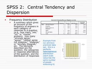
Central Tendency • Central tendency means the middle of the distribution. Three main indicators: • The Mode • The Median • The Mean
The Mode Defined • The most frequently occurring score or category • Most useful with categorical data. • Can be more than one mode (bimodal, etc.). • Unstable (based on limited scores). • To calculate: find the most frequently occurring score.
Calculating the Mode • 1122333455555556667789 • The mode is 5 because there are 7 fives in the distribution. • What is the mode for these data? • 12345677778889
The Median Defined • The middlemost score; separates the top 50 % of scores from the bottom 50% • More stable than the mode • Most useful for ordinal data
Calculating the Median – Even # of scores • If even number of scores, use the average of two middle scores • 1 2 3 4 5 6 7 8 (Order) • 2 2 3 3 4 5 5 6 (Number) • Median is 3.5 = (3+4)/2
Calculating Median (Even) • 1 2 3 4 5 6 7 8 (Order) • 1 2 2 2 2 3 3 3 (Number) • Median is 2 = (2+2)/2 • 1 2 3 4 5 6 7 8 9 10 (Order) • 1 2 2 5 6 8 9 9 9 10 (Number) • Median is 7 = (6+8)/2
Calculating Median (Odd) • If there are an odd number of scores in the distribution, the median is the middle score [(N+1)/2]. • 1 2 3 4 5 6 7 8 9 (Order) • 1 2 4 5 8 9 9 9 10 (Number) • Median is 8 (fifth score)[(9+1)/2]
Calculating Median (Test) • What is the median? • 1 2 3 4 5 6 7 8 9 (Order) • 2 3 4 5 6 8 9 9 9 (Number) • 1 2 3 4 5 6 (Order) • 0 5 7 9 9 9 (Number)
The Mean Defined • The mean is the arithmetic average. It is the sum of scores divided by the number of scores. • That is, add ‘em all up and divide by how many you’ve got.
Mean Defined • In the sample, the mean is: • In the population, the mean is:
Properties of the Mean • Stable • Basis for many statistical procedures • Unbiased estimator – will not over or underestimate population mean on average. • Deviations from mean sum to zero.
Calculating the Mean • 1 2 3 4 5 • Mean is (1+2+3+4+5)/5 = 15/5 = 3 • 2 2 2 3 3 3 • Mean is (2+2+2+3+3+3) = 15/6 = 2+3/6 = 2.5
Comparing Measures of Central Tendency • Use mode when • Need speed – fastest • Need score that occurs most often • Use Median when • Have small but skewed distribution • Missing/arbitrarily determined scores • Use Mean when • Estimating the population mean
Dispersion Defined • Dispersion refers to the spread of scores around the mean. Hug or hate the mean. • Four main indices of dispersion: • Range • Average Deviation • Variance • Standard Deviation
The Range • The Range is the difference between the top and bottom scores (Max – min). • Gives a quick approximation of variability in the data • Depends on quality of extreme scores
Calculating the Range • What is the range? • 1 2 2 3 3 5 6 7 8 9 • The range is 9-1 = 8. • 5 7 9 12 • The range is 12-5 = 7. • 2 2 2 2 3 3 3 4 4 13 • The range is 13-2 = 11.
Average Deviation Defined • The average deviation is the average absolute difference between the scores and the mean. • The formula for the AD is:
Calculating the AD • To find the Average Deviation • Find the mean • Subtract the mean from each score • Take the absolute value of the difference • Sum the absolute values • Divide by N, the number of scores
Calculating the AD • Example of AD • 2 2 3 3 4 4 • Mean is 3 = (18/6) • Absolute deviations: 1 1 0 0 1 1 • Sum is 4 • AD is 4/6 = 2/3 = .67 • Nice conceptually, but not very useful in practice
Variance Defined • The average of the unsigned deviations is zero • The average of the absolute deviations is bigger than zero unless all observations are at the mean • Instead of taking absolute value, we can square the deviations
Variance Defined • The variance is the average or mean of the squared deviations. • The population formula: • The sample formula:
Calculating the Variance • From the last slide, the sum of squared deviations is 8. • The average is 8/3 = 2.67 • This is the variance.
Calculating the Variance • What is the variance of the following distribution? • 5 6 7 8 9 10 • Answer: 2.92
Calculating the Variance • For reasons we will describe later, SPSS calculates the sample variance like this: • The only difference is (N-1) instead of N. You need this to compare your answer to SPSS. Use N-1 to compare to SPSS so you agree.
Standard Deviation Defined • The standard deviation is the square root of the variance. • The variance is the average squared deviation. • The standard deviation is in the original, unsquared units of measurement. • It’s easier to interpret than the variance.
Standard Deviation Defined • The population formula: • The sample formula {SPSS uses (N-1)}:
A Look Ahead • The mean, variance and standard deviation form the basis of most of the statistics we will be using. • If we do an experiment, we will look at the means and variance to decide if the treatment had an effect.
Using SPSS • Next we will wake up SPSS and see how to get it to provide the estimates of central tendency and variability
Homework • Compute estimates of central tendency (mode, median, mean). • Compute estimates of variability (range, variance, SD). • Explain them. • Compare the two distributions. • Due at the beginning of next lab.