Large scale structure in the SDSS
Large scale structure in the SDSS. The ISW effect The Ly-alpha forest Galaxies and Clusters Marked correlations: There’s more to the points Ravi K. Sheth (UPitt/UPenn). The ISW effect. Cross-correlate CMB and galaxy distributions Interpretation requires understanding of galaxy population.

Large scale structure in the SDSS
E N D
Presentation Transcript
Large scale structure in the SDSS • The ISW effect • The Ly-alpha forest • Galaxies and Clusters • Marked correlations: There’s more to the points Ravi K. Sheth (UPitt/UPenn)
The ISW effect Cross-correlate CMB and galaxy distributions Interpretation requires understanding of galaxy population
Expected scaling of signal Expect NO signal in Einstein de-Sitter! Recent (2003) detections in X-ray and radio-selected catalogs
Cross-correlate LRGs with CMB Measured signal combination of ISW and SZ effects Estimate both using halo model (although signal dominated by linear theory); Signal predicted to depend on b(a) D(a) d/dt [D(a)/a]
Evolution and bias Work in progress to disentangle evolution of bias from z dependence of signal (Scranton et al. 2004)
Spherical harmonic analysis similar (Padmanabhan et al 2004)
The Ly-a forest • Evolution measured over 2.2<z<4.2 • Consistent with WMAP LCDM cosmology (hi-z universe ~ EdS) • Series of papers by McDonald, Seljak et al. (2004) • (Alternative analysis by Hui et al. 200?)
Spatial Clustering • Large scale measurements can detect baryon wiggles/bump: • LRG clustering • QSO clustering • Smaller scale measurements constrain galaxy formation models
Kauffmann, Diaferio, Colberg & White 1999 Also Cole et al., Benson et al., Somerville & Primack, Colin et al. Colors indicate age
Halo-model of galaxy clustering • Two types of pairs: only difference from dark matter is that now, number of pairs in m-halo is not m2 • ξdm(r) =ξ1h(r) + ξ2h(r) • Spatial distribution within halos is small-scale detail
Comparison with simulations Sheth et al. 2001 steeper • Halo model calculation of x(r) • Red galaxies • Dark matter • Blue galaxies • Note inflection at scale of transition from 1-halo term to 2-halo term • Bias constant at large r shallower x1h›x2h x1h‹x2h →
Power-law: x(r) = (r0/r)g slope g = -1.8 Totsuji & Kihara 1969
Not a power law Feature on few Mpc scale; expected as transition from 1halo to 2halo term (Zehavi et al. 2004)
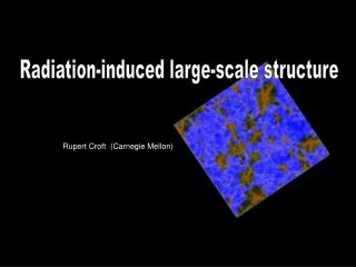
N-body simulations of gravitational clustering in an expanding universe Lots of substructure! (Model by Lee 2004)
Galaxies and halo substructure • Better to think in terms of center + satellite: g1(m) = 1 + [m/23m1(L)]a(L) for m>m1(L) • Higher order moments from assumption that satellite distribution is Poisson • Poisson model consistent with assumption that halo substructure = galaxies
Color dependence and cross-correlations consistent with simplest halo model
fingers of god Redshift space trends qualitatively consistent with v2 ~ m2/3 scaling—quantitative agreement also?
Galaxy formation models ~ correctly identify the halos in which galaxies formGalaxy ~ halo substructure is reasonable model
Extensions • Poisson model implies a complete model of point distribution • Can now make mock catalogs that have correct LF and 2pt function---check using n-pt, Minkowski’s,… • Assume monotonic relation between subclump mass and galaxy luminosity to get L-s relations • Include correlations between L, size, color, etc. • Relate galaxy distribution to cluster distribution (what is better tracer of mass: L? Ngal? S?) • Model of BCGs (e.g. use C4 catalog)
Successes and Failures • Distribution of sizes ~ Lognormal: seen in SDSS • Morphology-density relation (oldest stars in clusters/youngest in field) • Type-dependent clustering: red galaxies have steep correlation function; clustering strength increases with luminosity • Distribution of luminosities • Correlations between observables (luminosity/color, luminosity/velocity dispersion)
Sizes of disks and bulges Observed distribution ~ Lognormal Distribution of halo spins ~ Lognormal Distribution of halo concentrations ~ Lognormal (Bernardi et al. 2003; Kauffmann et al. 2003; Shen et al. 2003)
Environmental effects • Fundamental assumption: all environmental trends come from fact that massive halos populate densest regions
Color and Luminosity Hogg et al. 2004
Density and Lumi-nosity Hogg et al. 2004
Marked correlation functions Weight galaxies by some observable (e.g. luminosity, color, SFR) when computing clustering statistics (standard analysis weights by zero or one)
There’s more to the point(s) • Multi-band photometry becoming the norm • CCDs provide accurate photometry; possible to exploit more than just spatial information • How to estimate clustering of observables, over and above correlations which are due to spatial clustering? • Do galaxy properties depend on environment? Standard model says only dependence comes from parent halos…
Early-type galaxies • Models suggest cluster galaxies older, redder, more massive • Weak, if any, trends seen
Marked correlations (in volume-limited catalogs) Close pairs are redder, and have larger D4000, suggesting they are older, even though no strong trend seen with s Environment matters! hi-z low-z D4000
Marked correlations (usual correlation function analysis sets m = 1 for all galaxies) W(r) is a ‘weighted’ correlation function, so … marked correlations are related to weighted ξ(r)
Luminosity as a mark • Mr from SDSS • BIK from semi-analytic • model • Little B-band light • associated with • close pairs; more B-band • light in ‘field’ than ‘clusters’ • Vice-versa in K • Feature at 3/h Mpc in all • bands: Same physical • process the cause? • e.g. galaxies form in groups • at the outskirts of clusters
Colors and star formation • Close pairs tend to be redder • Scale on which feature • appears smaller at higher z: • clusters smaller at high-z? • Amplitude drops at lower z: • close red pairs merged? • Close pairs have small • star formation rates; scale • similar to that for color even • though curves show • opposite trends! • Same physics drives both • color and SFR?
Stellar mass • Circles show M*, crosses show LK • Similar bumps, wiggles in both: offset related to rms M*, L • Evolution with time: M* grows more rapidly in dense regions
Halo-model of marked correlations Again, write in terms of two components: W1gal(r) ~∫dm n(m) g2(m)‹W|m›2ξdm(m|r)/rgal2 W2gal(r) ≈ [∫dm n(m) g1(m) ‹W|m›b(m)/rgal]2ξdm(r) So, on large scales, expect 1+W(r) 1+ξ(r) 1 + BWξdm(r) 1 + bgalξdm(r) M(r) = =
Most massive halos populate densest regions over-dense under-dense Key to understand galaxy biasing (Mo & White 1996; Sheth & Tormen 2002) n(m|d) = [1 + b(m)d] n(m)
Conclusions (mark these words!) • Marked correlations represent efficient use of information in new high-quality multi-band datasets (there’s more to the points…) • No ad hoc division into cluster/field, bright/faint, etc. • Comparison of SDSS/SAMs ongoing • test Ngalaxies(m); • then test if rank ordering OK; • finally test actual values • Halo-model is natural language to interpret/model