Download
1 / 19
190 likes | 310 Views
Hadronic showers in the SiW ECAL (with 2008 FNAL data). Philippe Doublet. Introduction. 2008 FNAL data used Pions of 2, 4, 6, 8 and 10 GeV Cuts on scintillator and Cherekov counters The SiW ECAL ~1 I : ½ of the hadrons interact 1x1 cm² pixels: tracking possibilities

E N D
Hadronic showers in the SiW ECAL (with 2008 FNAL data) Philippe Doublet Philippe Doublet (LAL)
Introduction • 2008 FNAL data used • Pions of 2, 4, 6, 8 and 10 GeV • Cuts on scintillator and Cherekov counters • The SiW ECAL • ~1I: ½ of the hadrons interact • 1x1 cm² pixels:tracking possibilities • 30 layers with 3 different W depths 9 Si wafers
Procedure • Follow the MIP track • Find the interaction layer • Distinguish the types of interactions At low energies, finding the interaction and its type requires energy deposition and high granularity
InteractionFinder algorithm 1 • For « strong » interactions • Ei,Ei+1,Ei+2 > Ecut • Very simple and works very well at energies ~10 GeV • Does not really need high granularity but longitudinal segmentation helps X layer E(MIPs) Ecut layer
InteractionFinder algorithm 2 • For « weak » interactions • First criteria not satisfying (fails a lot when energy decreases) • Use the relative increase of energy: • (Ei+Ei+1)/(Ei-1+Ei-2) > Fcut • (Ei+1+Ei+2)/(Ei-1+Ei-2) > Fcut • Requires 5 layers: 2 before, 3 after (longitudinal segmentation) Y layer E(MIPs) Ecut (fails) layer
InteractionFinder algorithm 3 • Introduce classification: • Strong: « FireBall » class • Weak: 2 cases • If EiMIP-track neighbours / Ei > 0.5(prevents backscattering)Then « FireBall » class (transverse segmentation) • If (Ei+2+Ei+3)/(Ei-1+Ei-2) < Fcut(it was a local increase)Then « Peak » or « Pointlike » class (longitudinal segmentation) • If nothing, then « MIP » class Y layer E(MIPs) layer Pointlike interaction: πp scattering
Optimising Ecut and Fcut • Try interaction conditions for each event for a set of {Ecut,Fcut} • Fit the difference layer found – MC get σ and N (number of interactions found) • Trace for all combinations σ vs N • Get the best combination to get a small σ and a high N Found layer – MC layer
After optimisation • We care about the interactions found within +/- 1 layer (+/- 2 layers) w.r.t. the interaction layer in the MC +/- 1 layer +/- 2 layers David Ward’s results down to 8 GeV: ~70% inside +/- 1 layer 90% inside +/- 2 layers (Ecut criteria made a bit more complex: 3 out of 4 layers must satisfy cut)
Rates of interaction from 2 to 10 GeV: data vs MC (QGSP BERT) • After optimisation of Ecut and Fcut for each energy Nevts = 9599 Nevts = 12210 Nevts = 50509 Nevts = 48875 Nevts = 36292 Nevts = 85692 Nevts = 169723 Nevts = 114339 Nevts = 280310 Nevts = 136240 Good agreement between data and MC Data reconstruction and MC digitisation are official releases
A look at longitudinal and transverse profiles • Longitudinal profiles are drawn with 60 layers equivalent to those in the first stack (i.e. one layer in stack 2 is divided in 2 layers and one layer in stack 3 is divided in 3 layers) • Transverse size is calculated from the interaction point and weighted by the energy
Total longitudinal profiles: data vs MC (with shower structure) 2 GeV 4 GeV 6 GeV Reasonable agreement is found Blue = electrons contributions Green = protons Red = pions Black = others 8 GeV 10 GeV
Longitudinal profiles sorted by kind 10 GeV Total FireBall Obvious discrepancy with the MIP energies: Under investigation Maybe a problem of conversion MIPMeV in the official soft Peak MIP
Longitudinal profiles sorted by kind 2 GeV Total FireBall Mix of many contributions Still a good description at 2 GeV A lot of activity from protons in peak events Peak MIP
Total transverse profiles: data vs MC (QGSP BERT) 2 GeV 4 GeV 6 GeV Radius (mm) Good agreement: MIP peak and hadron peak clearly well identified 8 GeV 10 GeV Error in run selection seen, being corrected
Transverse profiles sorted by kind 10 GeV Total FireBall Peaks in the total histogram well separated. Thanks to granularity « MIP » and « Peak » are distinguished. Peak MIP
Transverse profiles sorted by kind 2 GeV Total FireBall Peak Separation slightly worse but still good at 2 GeV. MIP
Another interesting feature • « MIP » events contain two kind of events • They can be separated and classified into REAL MIPs and pion scattering using the extrapolated MIP track (transverse segmentation) development of some particle flow technique seem possible layer 5 cm ! layer
Conclusion • We combine energyandhigh granularity to classify hadronic interactions and even see them clearly • The transverse profiles agree very well • The longitudinal profiles are slightly higher for MC certainly due to a conversion factor problem • The 3 types of interaction allow to separate clearly the profiles and another can even be identified • Results stable obtained with official releases • Other physics lists available • CAN note in preparation to be ready for CALOR2010
Software versions (all official) • For reconstruction of FNAL runs (done by Alexander Kaplan): • Calice_userlib v04-10 • Calice_reco v04-06 • For digitisation of MC samples (done by Lars Weuste): • Calice_userlib v04-10 • Calice_reco v04-06 Same versions