Image segmentation
Image segmentation. The goals of segmentation. Group together similar-looking pixels for efficiency of further processing “Bottom-up” process Unsupervised. “superpixels”. X. Ren and J. Malik. Learning a classification model for segmentation. ICCV 2003. The goals of segmentation.
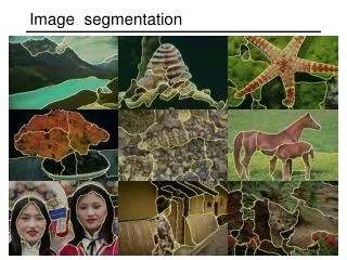

Image segmentation
E N D
Presentation Transcript
The goals of segmentation • Group together similar-looking pixels for efficiency of further processing • “Bottom-up” process • Unsupervised “superpixels” X. Ren and J. Malik. Learning a classification model for segmentation. ICCV 2003.
The goals of segmentation • Separate image into coherent “objects” • “Bottom-up” or “top-down” process? • Supervised or unsupervised? human segmentation image Berkeley segmentation database:http://www.eecs.berkeley.edu/Research/Projects/CS/vision/grouping/segbench/
Inspiration from psychology • The Gestalt school: Grouping is key to visual perception The Muller-Lyer illusion http://en.wikipedia.org/wiki/Gestalt_psychology
The Gestalt school • Elements in a collection can have properties that result from relationships • “The whole is greater than the sum of its parts” occlusion subjective contours familiar configuration http://en.wikipedia.org/wiki/Gestalt_psychology
Emergence http://en.wikipedia.org/wiki/Gestalt_psychology
Grouping phenomena in real life Forsyth & Ponce, Figure 14.7
Grouping phenomena in real life Forsyth & Ponce, Figure 14.7
Gestalt factors • These factors make intuitive sense, but are very difficult to translate into algorithms
Segmentation as clustering Source: K. Grauman
Segmentation as clustering • K-means clustering based on intensity or color is essentially vector quantization of the image attributes • Clusters don’t have to be spatially coherent Image Intensity-based clusters Color-based clusters
Segmentation as clustering Source: K. Grauman
Segmentation as clustering • Clustering based on (r,g,b,x,y) values enforces more spatial coherence
K-Means for segmentation • Pros • Very simple method • Converges to a local minimum of the error function • Cons • Memory-intensive • Need to pick K • Sensitive to initialization • Sensitive to outliers • Only finds “spherical” clusters
Mean shift clustering and segmentation • An advanced and versatile technique for clustering-based segmentation http://www.caip.rutgers.edu/~comanici/MSPAMI/msPamiResults.html D. Comaniciu and P. Meer, Mean Shift: A Robust Approach toward Feature Space Analysis, PAMI 2002.
Mean shift algorithm • The mean shift algorithm seeks modes or local maxima of density in the feature space Feature space (L*u*v* color values) image
Mean shift Searchwindow Center of mass Mean Shift vector Slide by Y. Ukrainitz & B. Sarel
Mean shift Searchwindow Center of mass Mean Shift vector Slide by Y. Ukrainitz & B. Sarel
Mean shift Searchwindow Center of mass Mean Shift vector Slide by Y. Ukrainitz & B. Sarel
Mean shift Searchwindow Center of mass Mean Shift vector Slide by Y. Ukrainitz & B. Sarel
Mean shift Searchwindow Center of mass Mean Shift vector Slide by Y. Ukrainitz & B. Sarel
Mean shift Searchwindow Center of mass Mean Shift vector Slide by Y. Ukrainitz & B. Sarel
Mean shift Searchwindow Center of mass Slide by Y. Ukrainitz & B. Sarel
Mean shift clustering • Cluster: all data points in the attraction basin of a mode • Attraction basin: the region for which all trajectories lead to the same mode Slide by Y. Ukrainitz & B. Sarel
Mean shift clustering/segmentation • Find features (color, gradients, texture, etc) • Initialize windows at individual feature points • Perform mean shift for each window until convergence • Merge windows that end up near the same “peak” or mode
Mean shift segmentation results http://www.caip.rutgers.edu/~comanici/MSPAMI/msPamiResults.html
Mean shift pros and cons • Pros • Does not assume spherical clusters • Just a single parameter (window size) • Finds variable number of modes • Robust to outliers • Cons • Output depends on window size • Computationally expensive • Does not scale well with dimension of feature space
j wij i Images as graphs • Node for every pixel • Edge between every pair of pixels (or every pair of “sufficiently close” pixels) • Each edge is weighted by the affinity or similarity of the two nodes Source: S. Seitz
j wij i Segmentation by graph partitioning • Break Graph into Segments • Delete links that cross between segments • Easiest to break links that have low affinity • similar pixels should be in the same segments • dissimilar pixels should be in different segments A B C Source: S. Seitz
Measuring affinity • Suppose we represent each pixel by a feature vector x, and define a distance function appropriate for this feature representation • Then we can convert the distance between two feature vectors into an affinity with the help of a generalized Gaussian kernel:
Scale affects affinity • Small σ: group only nearby points • Large σ: group far-away points
Graph cut • Set of edges whose removal makes a graph disconnected • Cost of a cut: sum of weights of cut edges • A graph cut gives us a segmentation • What is a “good” graph cut and how do we find one? B A Source: S. Seitz
Minimum cut • We can do segmentation by finding the minimum cut in a graph • Efficient algorithms exist for doing this Minimum cut example
Minimum cut • We can do segmentation by finding the minimum cut in a graph • Efficient algorithms exist for doing this Minimum cut example
Cuts with lesser weight than the ideal cut Ideal Cut Normalized cut • Drawback: minimum cut tends to cut off very small, isolated components * Slide from Khurram Hassan-Shafique CAP5415 Computer Vision 2003
Normalized cut • Drawback: minimum cut tends to cut off very small, isolated components • This can be fixed by normalizing the cut by the weight of all the edges incident to the segment • The normalized cut cost is: • w(A, B) = sum of weights of all edges between A and B J. Shi and J. Malik. Normalized cuts and image segmentation. PAMI 2000
Normalized cut • Let W be the adjacency matrix of the graph • Let D be the diagonal matrix with diagonal entries D(i, i) = Σj W(i, j) • Then thenormalized cut cost can be written aswhere y is an indicator vector whose value should be 1 in the ith position if the ith feature point belongs to A and a negative constant otherwise J. Shi and J. Malik. Normalized cuts and image segmentation. PAMI 2000
Normalized cut • Finding the exact minimum of the normalized cut cost is NP-complete, but if we relaxy to take on arbitrary values, then we can minimize the relaxed cost by solving the generalized eigenvalue problem (D − W)y =λDy • The solution y is given by the generalized eigenvector corresponding to the second smallest eigenvalue • Intutitively, the ith entry of y can be viewed as a “soft” indication of the component membership of the ith feature • Can use 0 or median value of the entries as the splitting point (threshold), or find threshold that minimizes the Ncut cost
Normalized cut algorithm • Represent the image as a weighted graph G = (V,E), compute the weight of each edge, and summarize the information in D and W • Solve (D − W)y = λDy for the eigenvector with the second smallest eigenvalue • Use the entries of the eigenvector to bipartition the graph • To find more than two clusters: • Recursively bipartition the graph • Run k-means clustering on values of several eigenvectors
Challenge • How to segment images that are a “mosaic of textures”?
Using texture features for segmentation • Convolve image with a bank of filters J. Malik, S. Belongie, T. Leung and J. Shi. "Contour and Texture Analysis for Image Segmentation". IJCV 43(1),7-27,2001.
Using texture features for segmentation • Convolve image with a bank of filters • Find textons by clustering vectors of filter bank outputs Image Texton map J. Malik, S. Belongie, T. Leung and J. Shi. "Contour and Texture Analysis for Image Segmentation". IJCV 43(1),7-27,2001.
Using texture features for segmentation • Convolve image with a bank of filters • Find textons by clustering vectors of filter bank outputs • The final texture feature is a texton histogram computed over image windows at some “local scale” J. Malik, S. Belongie, T. Leung and J. Shi. "Contour and Texture Analysis for Image Segmentation". IJCV 43(1),7-27,2001.
Pitfall of texture features • Possible solution: check for “intervening contours” when computing connection weights J. Malik, S. Belongie, T. Leung and J. Shi. "Contour and Texture Analysis for Image Segmentation". IJCV 43(1),7-27,2001.
Results: Berkeley Segmentation Engine http://www.cs.berkeley.edu/~fowlkes/BSE/