Section 12 Air Quality Forecasting Tools
Section 12 Air Quality Forecasting Tools. Background. Forecasting tools provide information to help guide the forecasting process. Forecasters use a variety of data products, information, tools, and experience to predict air quality.


Section 12 Air Quality Forecasting Tools
E N D
Presentation Transcript
Background • Forecasting tools provide information to help guide the forecasting process. • Forecasters use a variety of data products, information, tools, and experience to predict air quality. • Forecasting tools are built upon an understanding of the processes that control air quality. • Forecasting tools: • Subjective • Objective • More forecasting tools = better results. www.epa.vic.gov.au/air/AAQFS Section 12 – Air Quality Forecasting Tools
Fewer resources, lower accuracy More resources, potential for higher accuracy Background • Persistence • Climatology • Criteria • Statistical • Classification and Regression Tree (CART) • Regression • Neural networks • Numerical modeling • Phenomenological and experience • Predictor variables Section 12 – Air Quality Forecasting Tools
Selecting Predictor Variables (1 of 3) • Many methods require predictor variables. • Meteorological • Air Quality • Before selecting particular variables it is important to understand the phenomena that affect pollutant concentrations in your region. • The variables selected should capture the important phenomena that affect pollutant concentrations in the region. Section 12 – Air Quality Forecasting Tools
Selecting Predictor Variables (2 of 3) • Select observed and forecasted variables. Predictor variables can consist of observed variables (e.g., yesterday’s ozone or PM2.5 concentration) and forecasted variables (e.g., tomorrow’s maximum temperature). • Make sure that predictor variables are easily obtainable from reliable source(s) and can be forecast. • Consider uncertainty in measurements, particularly measurements of PM. Section 12 – Air Quality Forecasting Tools
Selecting Predictor Variables (3 of 3) • Begin with as many as 50 to 100 predictor variables. • Use statistical analysis techniques to identify the most important variables. • Cluster analysis is used to partition data into similar and dissimilar subsets. Unique (i.e., dissimilar) variables should be used to avoid redundancy. • Correlation analysis is used to evaluate the relationship between the predictand (i.e., pollutant levels) and various predictor variables. • Step-wise regression is an automatic procedure that allows the statistical software (SAS, Statgraphics, Systat, etc.) to select the most important variables and generate the best regression equation. • Human selectionis another means of selecting the most important predictor variables. Section 12 – Air Quality Forecasting Tools
Common Ozone Predictor Variables Section 12 – Air Quality Forecasting Tools
Common PM2.5 Predictor Variables Section 12 – Air Quality Forecasting Tools
Assembling a dataset • Determine what data to use • What data types are needed and available • What sites are representative • What air quality monitoring network(s) to use (for example, continuous versus passive or filter) • What type of meteorological data are available (surface, upper-air, satellite, etc.) • How much data is available (years) Section 12 – Air Quality Forecasting Tools
Assembling a dataset • Acquire historical data including • Hourly pollutant data • Daily maximum pollutant metrics, such as • Peak 1-hr ozone • Peak 8-hr average ozone • 24-hr average PM2.5 or PM10 • Hourly meteorological data • Radiosonde data • Model data • Meteorological outputs • MM5/TAPM • Other • Surface and upper-air weather charts • HYSPLIT trajectories Section 12 – Air Quality Forecasting Tools
Assembling a dataset • Quality control data • Check for outliers • Look at the minimum and maximum values for each field; are they reasonable? • Check rate of change between records at each extreme. • Time stamps • Has all data been properly matched by time? • Time series plots can help identify problems shifting from UTC to LST. • Missing data • Is the same identifier used for each field? I.e., –999. • Units • Are units consistent among different data sets? I.e., m/s or knots for wind speeds. • Validation codes • Are validation codes consistent among different data sets? • Do the validation codes match the data values? I.e., are data values of –999 flagged as missing? Section 12 – Air Quality Forecasting Tools
Forecasting Tools and Methods(1 of 2) Tool development is a function of • Amount and quality of data (air quality and meteorological) • Resources for development • Human • Software • Computing • Resources for operations • Human • Software • Computing Section 12 – Air Quality Forecasting Tools
Forecasting Tools and Methods(2 of 2) For each tool • What is it? • How does it work? • Example • How to develop it? • Strengths • Limitations Ozone = WS * 10.2 +… Section 12 – Air Quality Forecasting Tools
Persistence (1 of 2) • Persistence means to continue steadily in some state. • Tomorrow’s pollutant concentration will be the same as Today’s. • Best used as a starting point and to help guide other forecasting methods. • It should not be used as the only forecasting method. • Modifying a persistence forecast with forecasting experience can help improve forecast accuracy. Persistence forecast Section 12 – Air Quality Forecasting Tools
Persistence (2 of 2) • Seven high ozone days (red) • Five of these days occurred after a high day (*) • Probability of high ozone occurring on the day after a high ozone day is 5 out of 7 days • Probability of a low ozone day occurring after a low ozone day are 20 out of 22 days • Persistence method would be accurate 25 out of 29 days, or 86% of the time Peak 8-hr ozone concentrations for a sample city Section 12 – Air Quality Forecasting Tools
Persistence – Strengths • Persistence forecasting • Useful for several continuous days with similar weather conditions • Provides a starting point for an air quality forecast that can be refined by using other forecasting methods • Easy to use and requires little expertise Section 12 – Air Quality Forecasting Tools
Persistence – Limitations • Persistence forecasting cannot • Predict the start and end of a pollution episode • Work well under changing weather conditions when accurate air quality predictions can be most critical Section 12 – Air Quality Forecasting Tools
Climatology • Climatology is the study of average and extreme weather or air quality conditions at a given location. • Climatology can help forecasters bound and guide their air quality predictions. Section 12 – Air Quality Forecasting Tools
Climatology – Example Average number of days per month with ozone in each AQI category for Sacramento, California Section 12 – Air Quality Forecasting Tools
Developing Climatology • Create a data set containing at least five years of recent pollutant data. • Create tables or charts for forecast areas containing • All-time maximum pollutant concentrations (by month, by site) • Duration of high pollutant episodes (number of consecutive days, hours of high pollutant each day) • Average number of days with high pollutant levels by month and by week • Day-of-week distribution of high pollutant concentrations • Average and peak pollutant concentrations by holidays and non-holidays, weekends and weekdays Section 12 – Air Quality Forecasting Tools
Developing Climatology • Consider emissions changes • For example, fuel reformulation • It may be useful to divide the climate tables or charts into “before” and “after” periods for major emissions changes. McCarthy et al., 2005 Section 12 – Air Quality Forecasting Tools
Day of week distribution of high PM2.5 days Climatology • High pollution days occur most often on Wednesday • High pollution days occur least often at the beginning of the week Section 12 – Air Quality Forecasting Tools
Climatology Distribution of high ozone days by upper-air weather pattern Section 12 – Air Quality Forecasting Tools
Climatology – Strengths • Climatology • Bounds and guides an air quality forecast produced by other methods • Easy to develop Section 12 – Air Quality Forecasting Tools
Climatology – Limitations • Climatology • Is not a stand-alone forecasting method but a tool to complement other forecast methods • Does not account for abrupt changes in emissions patterns such as those associated with the use of reformulated fuel, a large change in population, forest fires, etc. • Requires enough data (years) to establish realistic trends Section 12 – Air Quality Forecasting Tools
Criteria • Uses threshold values (criteria) of meteorological or air quality variables to forecast pollutant concentrations • For example, if temperature > 27°C and wind < 2 m/s then ozone will be in the Unhealthy AQI category • Sometimes called “rules of thumb” • Commonly used in many forecasting programs as a primary forecasting method or combined with other methods • Best suited to help forecast high pollution or low pollution events, or pollution in a particular air quality index category range rather than an exact concentration Section 12 – Air Quality Forecasting Tools
Criteria – Example Conditions needed for high pollution by month To have a high pollution day in July • maximum temperature must be at least 33C, • temperature difference between the morning low and afternoon high must be at least 11C • average daytime wind speed must be less than 3 m/s, • afternoon wind speed must be less than 4 m/s, and • the day before peak 1-hr ozone concentration must be at least 70 ppb. Lambeth, 1998 Section 12 – Air Quality Forecasting Tools
Developing Criteria (1 of 2) • Determine the important physical and chemical processes that influence pollutant concentrations • Select variables that represent the important processes • Useful variables may include maximum temperature, morning and afternoon wind speed, cloud cover, relative humidity, 500‑mb height, 850-mb temperature, etc. • Acquire at least three years of recent pollutant data and surface and upper-air meteorological data Section 12 – Air Quality Forecasting Tools
Developing Criteria (2 of 2) • Determine the threshold value for each parameter that distinguishes high and low pollutant concentrations. • For example, create scatter plots of pollutant vs. weather parameters. • Use an independent data set (i.e., a data set not used for development) to evaluate the selected criteria. Section 12 – Air Quality Forecasting Tools
Criteria – Strengths • Easy to operate and modify • An objective method that alleviates potential human biases • Complements other forecasting methods Section 12 – Air Quality Forecasting Tools
Criteria – Limitations • Selection of the variables and their associated thresholds is subjective. • It is not well suited for predicting exact pollutant concentrations. Section 12 – Air Quality Forecasting Tools
Classification and Regression Tree (CART) • CART is a statistical procedure designed to classify data into dissimilar groups. • Similar to criteria method; however, it is objectively developed. • CART enables a forecaster to develop a decision tree to predict pollutant concentrations based on predictor variables (usually weather) that are well correlated with pollutant concentrations. An example Cart tree for maximum ozone prediction for the greater Athens area. Section 12 – Air Quality Forecasting Tools
Ozone (Low–High) Temp high Temp low Moderate to High Moderate to Low WS - calm WS - strong WS -light WS - calm Low High Moderate Moderate Classification and Regression Tree (CART) Section 12 – Air Quality Forecasting Tools
CART – How It Works(1 of 2) The statistical software determines the predictor variables and the threshold cutoff values by • Reading a large data set with many possible predictor variables • Identifying the variables with the highest correlation with the pollutant • Continuing the process of splitting the data set and growing the tree until the data in each group are sufficiently uniform Section 12 – Air Quality Forecasting Tools
CART – How It Works (2 of 2) • To forecast pollutant concentrations using CARTs • Step through the tree starting at the first split and determine which of the two groups the data point belongs in, based on the cut-point for that variable; • Continue through the tree in this manner until an end node is reached. • The mean concentration shown in the end node is the forecasted concentration. • Note, slight differences in the values of predicted variables can produce significant changes in predicted pollutant levels when the value is near the threshold. Section 12 – Air Quality Forecasting Tools
CART – Example CART classification PM10 in Santiago, Chile Is the forecasted temperature at 850 mb 10.5°C? No Yes Node x Variable and criteria STD = Standard deviation Avg = Average PM10 (ug/m3) N = number of cases in node Variables: T850 - 12Z 850 MB temp DELTAP - the pressure difference between the base and top of the inversion MI0 - Synoptic weather potential (scale from 1-low to 5-high). FAVGTMP - 24-hour average temperature at La Paz FAVGRH - 24-hour average relative humidity at La Paz. Cassmassi, 1999 Section 12 – Air Quality Forecasting Tools
Developing CART • Determine the important processes that influence pollution. • Select variables that properly represent the important processes. • Create a multi-year data set of the selected variables. • Choose recent years that are representative of the current emission profile • Reserve a subset of the data for independent evaluation, but ensure it represents all conditions • Be sure variables are forecasted • Use statistical software to create a decision tree. • Evaluate the decision tree using the independent data set. Section 12 – Air Quality Forecasting Tools
CART – Strengths • Requires little expertise to operate on a daily basis; runs quickly. • Complements other subjective forecasting methods. • Allows differentiation between days with similar pollutant concentrations if the pollutant concentrations are a result of different processes. Since PM can form through multiple pathways, this advantage of CART can be particularly important to PM forecasting. Section 12 – Air Quality Forecasting Tools
CART – Limitations • Requires a modest amount of expertise and effort to develop. • Slight changes in predicted variables may produce large changes in the predicted concentrations. • CART may not predict pollutant concentrations during periods of unusual emissions patterns due to holidays or other events. • CART criteria and statistical approaches may require periodic updates as emission sources and land use changes. Section 12 – Air Quality Forecasting Tools
Regression Equations –How They Work (1 of 5) • Regression equations are developed to describe the relationship between pollutant concentration and other predictor variables • For linear regression, the common form isy = mx + b • At right, maximum temperature (Tmax) is a good predictor for peak ozone [O3] = 1.92*Tmax – 86.8 r = 0.77 r2 = 0.59 Section 12 – Air Quality Forecasting Tools
Regression Equations – How They Work (2 of 5) • More predictors can be added (“stepwise regression”) so that the equation looks like this: y = m1x1 + m2x2 + m3x3 + ……mnxn + b • Each predictor (xn) has its own “weight” (mn) and the combination may lead to better forecast accuracy. • The mix of predictors varies from place to place. Section 12 – Air Quality Forecasting Tools
Regression Equations – How They Work (3 of 5) Ozone Regression Equation for Columbus, Ohio 8hrO3 = exp(2.421 + 0.024*Tmax + 0.003*Trange - 0.006*WS1to6 + 0.007*00ZV925 - 0.004*RHSfc00 - 0.002*00ZWS500) Section 12 – Air Quality Forecasting Tools
Regression Equations – How They Work (4 of 5) • The various predictors are not equally weighted, some are more important than others. • It is essential to identify the strongest predictors and work hardest on getting those predictions right. Tmax vs. O3 Previous day O3 vs. O3 Wind Speed vs. O3 Section 12 – Air Quality Forecasting Tools
Regression Equations – How They Work (5 of 5) • In an example case, most of the variance in O3 is explained by Tmax (60%), with the additional predictors adding ~ 15%. • Overall, 75% of the variance in observed O3is explained by the forecast model. • Our job as forecasters is to fill in the additional 25% using other tools. Accumulated explained variance Section 12 – Air Quality Forecasting Tools
Developing Regression (1 of 2) • Determine the important processes that influence pollutant concentrations. • Select variables that represent the important processes that influence pollutant concentrations. • Create a multi-year data set of the selected variables. • Choose recent years that are representative of the current emission profile. • Reserve a subset of the data for independent evaluation, but ensure it represents all conditions. • Be sure variables are forecasted. • Use statistical software to calculate the coefficients and a constant for the regression equation. • Perform an independent evaluation of the regression model. Section 12 – Air Quality Forecasting Tools
Developing Regression (2 of 2) • Using the natural log of pollutant concentrations as the predictand may improve performance. • Do not to “over fit” the model by using too many prediction variables. An “over-fit” model will decrease the forecast accuracy. A reasonable number of variables to use is 5 to 10. • Unique variables should be used to avoid redundancy and co‑linearity. • Stratifying the data set may improve regression performance. • Seasons • Weekend vs. weekday Section 12 – Air Quality Forecasting Tools
Regression – Strengths • It is well documented and widely used in a variety of disciplines. • Software is widely available. • It is an objective forecasting method that reduces potential biases arising from human subjectivity. • It can properly weight relationships that are difficult to subjectively quantify. • It can be used in combination with other forecasting methods, or it can be used as the primary method. Section 12 – Air Quality Forecasting Tools
Regression – Limitations • Regression equations require a modest amount of expertise and effort to develop. • Regression equations tend to predict the mean better than the tails (i.e., the highest pollutant concentrations) of the distribution. They will likely underpredict the high concentrations and overpredict the low concentrations. • Regression criteria and statistical approaches may require periodic updates as emission sources and land use changes. • Regression equations require 3-5 years of measurement data in the region of application, including many instances of air pollution events, to develop. Section 12 – Air Quality Forecasting Tools
Neural Networks • Artificial neural networks are computer algorithms designed to simulate the human brain in terms of pattern recognition. • Artificial neural networks can be “trained” to identify patterns in complicated non-linear data. • Because pollutant formation processes are complex, neural networks are well suited for forecasting. • However, neural networks require about 50% more effort to develop than regression equations and provide only a modest improvement in forecast accuracy (Comrie, 1997). Section 12 – Air Quality Forecasting Tools
Neural Networks – How It Works • Neural networks use weights and functions to convert input variables into a prediction. • A forecaster supplies the neural network with meteorological and air quality data. • The software then weights each datum and sums these values with other weighted datum at each hidden node. • The software then modifies the node data by a non-linear equation (transfer function). • The modified data are weighted and summed as they pass to the output node. • At the output node, the software modifies the summed data using another transfer function and then outputs a prediction. Comrie, 1997 Section 12 – Air Quality Forecasting Tools