Download
1 / 123
1.25k likes | 1.78k Views
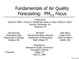
Fundamentals of Air Quality Forecasting: PM 2.5 Focus. Prepared by: Dianne S. Miller*, Clinton P. MacDonald, Adam N. Pasch, Patrick H. Zahn* Sonoma Technology, Inc. Petaluma, CA. Presented to: National Air Quality Conference Forecaster’s Training Dallas, TX March 2, 2009. Bill Ryan*

E N D
Fundamentals of Air Quality Forecasting: PM2.5 Focus Prepared by: Dianne S. Miller*, Clinton P. MacDonald, Adam N. Pasch, Patrick H. Zahn* Sonoma Technology, Inc. Petaluma, CA Presented to: National Air Quality Conference Forecaster’s Training Dallas, TX March 2, 2009 Bill Ryan* Pennsylvania State UniversityDepartment of Meteorology State College, PA Mike Gilroy Puget Sound Clean Air Agency Seattle, WA Clint Bowman Washington State Department of Ecology Olympia, WA * Presenter 905501.09-3580
Agenda • 12:30 – 12:35 Introduction • 12:35 – 12:55 Air quality overview • 12:55 – 1:35 Forecasting tools overview • 1:35 – 1:50 What controls air quality? • 1:50 – 2:30 Meteorology and its influence on air quality (part 1) • 2:30 – 3:00 Break • 3:00 – 4:50 Meteorology and its influence on air quality (part 2) • 4:50 – 5:00 Questions
Section 1: Air Quality Overview • What is in our air? • About PM2.5 • PM2.5 seasonal patterns • PM2.5 lifecycles and trends • PM2.5 formation and growth • PM2.5 monitoring • PM2.5 versus ozone
What Is In Our Air? • Mixture of invisible gases, particles, and water • Mostly nitrogen (78%) and oxygen (21%) • Remaining 1% contains • Argon • Water vapor • Carbon dioxide • Ozone • Particulate matter • And much more
About PM2.5 • A complex mixture of solid and liquid particles • Both a primary and secondary pollutant • Significant particle size variation • Seasonal and regional differences • Forms in many ways • Clean-air levels are <5 µg/m3 * • U.S. concentrations range from 0 to 200+ µg/m3 * • Health concerns Ultra-fine fly-ash or carbon soot "Night at Noon." London's Piccadilly Circus at midday during deadly smog episode in the winter of 1955.Source: When Smoke Ran Like Water, Devra Davis, Perseus Books *24-hr average
PM2.5 concentrations vary by season and region Average quarterly PM2.5 concentrations based on AIRNow data from 2005-2007 Seasonal Patterns – Regional/National (1 of 2) Jan-Mar Apr-Jun Oct-Dec July-Sept
Seasonal Patterns – Regional/National (2 of 2) Sulfate is important in the eastern U.S. while carbon and nitrate are important in the western U.S. (organic carbon mass)
Seasonal Patterns – Local • OM is the largest contributor to PM2.5 in the western U.S. in all months, with the highest contributions in the winter months. • Sulfates are a large contributor to PM2.5 in the eastern U.S. during the summer. • Nitrates increase in the winter months, with the most dramatic increases observed in the eastern U.S. Seattle – 5303300572002-2007 Cleveland – 390350060 2000-2006
Lifecycles and Trends • Lifecycles are daily and episodic changes in pollution levels. • Trends are long-term changes in air pollution that are caused by population and emission changes. • Importance • Daily forecasting (changes, evolution) • Communication (message, exposure) • Four time periods • Day/night (diurnal) and multi-day • Seasonal • Yearly • Long-term
In urban areas, during the afternoon, vertical mixing and horizontal transport tend to dilute concentrations. During the night and early morning, emissions are trapped by poor ventilation. In the afternoon, vertical mixing may carry pollutants above topographical barriers. During the night and early morning, dispersion may be hampered by topography. Lifecycles
In urban areas, winter mixing heights are low, trapping emissions. In the summer, intense vertical mixing raises mixing heights; higher mixing heights, in turn, tend to dilute concentrations. PM primary and precursor emissions are dependent upon seasonal energy consumption for heating and cooling, occurrence of fires, etc. Many gas-to-particle transformation rates are photochemically driven and peak in the summer. Summer Daytime Winter Daytime Trends – Seasonal Schichtel, 1999a
Formation Cloud/Fog Processes: Gases dissolve in a water droplet and chemically react. A solid particle exists when the water evaporates. Coagulation: Particles collide with each other and grow. NH4 SO2 Ammonium Sulfate Growth Condensation: Gases condense onto a small solid particle to form a bigger particle. Chemical Reaction: Gases react to form particles. Ammonium Nitrate NOx HNO3 + NH3 NH4NO3 (particle) Fn (Temp, RH) Nitric Acid Ammonia PM2.5 Formation and Growth
PM2.5 Monitoring Hourly PM2.5 monitoring network • Different PM2.5 monitors measure data at different time scales. • Continuous monitors measure data hourly. • Filter-based monitors measure data daily, every third day, or every sixth day.
PM2.5 versus Ozone • In some parts of the country, PM2.5 and ozone concentrations can be high at the same time. • In the Pacific Northwest, for example, PM2.5 concentrations are highest in the winter where ozone concentrations are the lowest.
Summary • PM2.5 is a complex mixture of chemicals from both primary emissions and secondary formation. • Diurnal, seasonal, and annual trends in PM2.5 are related to emission sources (and their temporal and seasonal patterns) and meteorology. • Forecasting PM2.5 is a challenge.
Section 2: Forecasting Tools • Persistence, trend • Climatology • Criteria, thresholds • Statistical • Classification and Regression Tree (CART) • Regression equations • Numerical modeling • Phenomenological and experience Fewer resources to develop, lower accuracy More resources to develop, potential for higher accuracy
Persistence, Trend • Persistence means to continue steadily in some physical state: “Tomorrow’s pollutant concentration will be the same as today’s.” • Trend means to continue to change at the same rate: “Today’s pollutant concentration increased 5 µg/m3 from yesterday’s; tomorrow’s pollutant concentration will increase 5 µg/m3 from today’s.” • Persistence and trend are used as starting points and guides for other forecasting methods. • Persistence and trend should not be used as the only forecasting methods.
Climatology (1 of 2) • Climatology is the study of average and extreme weather or air quality conditions at a given location. • Climatology can help forecasters bound and guide their air quality predictions. • All-time maximum pollutant concentrations (by month, by site) • Duration of high pollutant episodes (number of consecutive days, hours of high pollutant concentrations each day) • Average number of days with high pollutant levels by month and by week • Day-of-week distribution of high pollutant concentrations • Average and peak pollutant concentrations by holidays and non-holidays, weekends and weekdays
Number of days Climatology (2 of 2) Sacramento, CA Daily record maximum PM2.5 concentration Birmingham, AL Day of week distribution of high PM2.5 days (2001-2004) Columbus, OHPM2.5 episode length (2003-2007) Number of episodes colors represent AQI levels
Criteria, Thresholds • Use threshold values of meteorological or air quality variables to forecast pollutant concentrations: “If temperature > 27°C and wind speed < 2 m/s, then ozone will be in the Unhealthy AQI category.” • Best suited to help forecast high pollution or low pollution events, or pollution in a particular AQI category range. • Not ideal for an exact concentration forecast
PM2.5 (Low–High) Temp low Temp high Moderate to High Moderate to Low WS - calm WS - strong WS -light WS - calm Low High Moderate Moderate Classification and Regression Tree (CART) • A statistical procedure designed to classify data into distinct (or dissimilar) groups • Enables a forecaster to use a decision tree to predict pollutant concentrations based on the values of predictor variables.
Numerical Modeling • Mathematically represents the spatial and temporal evolution of processes that affect pollution using the laws of physics. • Requires a system of models to simulate the emission, transport, diffusion, transformation, and removal of air pollution • Numerical weather models • Emissions models • Air quality models
Numerical Weather Models Provide weather predictions forward in time, given an initial starting point (an initialization). Initialization (t = 0 hours) Forecast (t = 24 hours)
Numerical Weather Models – Outputs • Graphical output (spatial images) used for daily forecasting • Surface • Highs and lows • Fronts • Wind direction and speed • Precipitation • 850 mb • Troughs and ridges • Wind • Temperature advection • 700 mb • Relative humidity • Vertical velocity • 500 mb • Large-scale troughs or ridges • Small-scale pressure waves
Numerical Weather Models – Types (1 of 3) • RUC (Rapid Update Cycle) • NAM (North American Meso) • GFS (Global Forecast System) • Other models not discussed here are • NGM (Nested Grid Model—will be terminated Mar 2009) • UK Met • ECMWF (European) • Canadian
Numerical Weather Models – Types (2 of 3) • Rapid Update Cycle (RUC) model • 13-km grid • 50 vertical levels • Runs hourly • Forecasts out 9 hours in hourly increments • North American Meso (NAM) model • Driven by the Weather Research Forecast (WRF) model • 12-km grid • 60 vertical levels • Runs 4 times per day • Forecasts out 84 hours in 3-hr increments
Numerical Weather Models – Types (3 of 3) • Global Forecast System (GFS) model • 0.5-1-degree grid (~40-100 km) • 64 vertical levels • Runs 4 times per day • Forecasts out to 16 days (384 hours) in 6-hr increments
Air Quality Models – NOAA/EPA Air Quality Forecasts • Twice daily national ozone forecasts at 12-km resolution driven by Community Multiscale Air Quality (CMAQ) Modeling System • National smoke predictionsat 12-km resolution • PM2.5 prediction capability in developmental stage but still a few years from operational deployment
Air Quality Models – Real-time BlueSky Gateway Modeling System • Experimental predictions of PM2.5 resulting from fire and non-fire sources on a national scale • Smoke prediction enabled by the USFS BlueSky Framework • Work supported by NASA Decision Support, USFS, and the Joint Fire Science Program http://www.getbluesky.org/bluesky/sti
Air Quality Models – Canadian Air Quality Forecasts • CHRONOS (Canadian Hemispheric and Regional Ozone and NOx System) • Once daily (00Z) PM2.5 and ozone forecasts over U.S. and Canada at 21-km resolution • To be replaced by 15-km GEM-MACH operational model (2009?) http://www.weatheroffice.gc.ca/chronos/index_e.html
Air Quality Observational Tools – IDEA • IDEA – Infusing Satellite Data into Environmental Applications • NASA-NOAA-EPA partnership to improve air quality assessment, management, and prediction • MODIS aerosol optical depth retrievals fused into EPA/NOAA analyses for public benefit • Tutorials on product interpretation available on website http://www.star.nesdis.noaa.gov/smcd/spb/aq/index.php
Ws, T, O3 Phenomenological and Experience • Involves analyzing and conceptually processing air quality and meteorological information to formulate an air quality prediction • Heavily relies on the experience provided by a meteorologist or air quality scientist who understands the phenomena that influence pollution • Balances some of the limitations of objective prediction methods
Phenomenological Guidelines – Example • Knowledge can be documented as forecast rules
Phenomenological – Forecast Worksheets Example forecast worksheets for PM2.5 35 40 20
Summary • Many types of forecast tools can be used in a forecast program. • Many national tools are already available • Custom, city-specific tools can be developed • Tools range from simple to complex • Tools can be subjective or objective • A suite of forecast tools will improve accuracy.
Meteorology (Weather) Chemistry Emissions Section 3: What Controls Air Quality? • Emissions • Chemistry • Weather
Meteorology Chemistry Emissions Emissions – What Are They? • Man-made sources (anthropogenic) • NOx through combustion • VOCs and particulate carbon through combustion and numerous other sources • SO2 through combustion of coal and oil that contains sulfur • Metals through industrial processes • PM through combustion, mechanical processes (e.g., wind blown dust through human activity) • Natural sources (biogenic) • VOCs from trees/vegetation • NOx from soils (fertilizer)
Wind speed (WS) Concentration ES/WS ES Vertical mixing (VM) ES Concentration ES/VM Emissions Impact • Pollutant concentration depends on • Emissions source (ES) location, source density, and source strength • Meteorology Courtesy of New Jersey Department of Environmental Protection
Primary PM2.5 (directly emitted) Ca, Si, Fe, Al (dust) Sea salt (Na, Cl) Organic matter (OM) Elemental carbon (EC) Zn, Fe, Pb (industrial) Small amounts of sulfate and nitrate Secondary PM2.5 (precursor gases that form PM2.5 in the atmosphere) Sulfur dioxide (SO2): forms sulfates Nitrogen oxides (NOx): forms nitrates Ammonia (NH3): forms ammonium compounds Volatile organic compounds (VOCs): contribute to OM Meteorology Chemistry Emissions PM2.5 Chemistry (1 of 2) PM2.5 is composed of a mixture of primary and secondary compounds.
PM2.5 Chemistry (2 of 2) • Sulfate formation in the atmosphere • Photochemical oxidation of sulfur dioxide (SO2) in the daytime forms sulfates (SO4) • Condensation of sulfuric acid (H2SO4) results in the accumulation and growth of sulfate particles [(NH4)2SO4] • Sulfate formation in clouds • SO2 is scavenged by water droplets and oxidizes to form sulfate • Cloud droplets evaporate, leaving sulfate residue • Nitrate formation • Photochemical reaction of nitrogen dioxide (NO2) with hydroxyl radicals (OH) will form nitric acid (HNO3) in the daytime • NO2 will react with ozone at night to form HNO3 • HNO3 reacts with ammonia to form ammonium nitrate particles (NH4NO3) Summer Winter
Meteorology Chemistry Emissions Global Synoptic Mesoscale Urban Neighborhood PM2.5 Weather • Processes that influence air quality • Sunlight • Horizontal dispersion • Vertical mixing • Transport • Clouds and precipitation • Large scale to local scale • Global – 4,000 km – 20,000 km • Synoptic – 400 km – 4,000 km • Meso – 10 km – 400 km • Urban – 5 km – 50 km • Neighborhood – 50 m – 5 km Local Scale
Summary • Forecasters need to understand • PM and PM precursor emissions • Atmospheric chemistry related to PM formation and removal • Weather’s contributions to pollutant chemistry, dispersion, and transport
Section 4: Meteorological Phenomena • What phenomena are important for air quality forecasting? • Meteorological variables • Temperature • Water vapor • Pressure • Meteorological phenomena • Surface pressure patterns and regional/local winds • Aloft pressure patterns • Fronts and air masses • Stability and mixing • Clouds, fog, and precipitation
Meteorological Variables • These variables • Define the state of the atmosphere • Are predicted by all weather models • Directly or indirectly affect chemical reactions, emissions, dispersion, transport, and deposition • Different formulations/analyses of these variables let forecasters predict different weather phenomena
Temperature • Temperature is an important variable that affects PM2.5 formation, emissions, dispersion, and transport • At lower temperatures, there is more home heating (residential wood burning) • Higher temperatures promote more volatilization of VOCs and increased biogenic emissions • Forecasters are interested in changes in temperature vertically (e.g., inversions), spatially (e.g., fronts), and temporally (e.g., diurnal mixing heights)
Water Vapor • Water vapor (a.k.a. moisture) can increase • Production of secondary PM2.5 including sulfates and nitrates in some areas • Deposition in the form of precipitation • Forecasters are interested in changes in water vapor content temporally (e.g., diurnal relative humidity changes) and vertically (e.g., cloud formation potential).
Water Vapor Parameters • Dew Point Temperature • The temperature to which a given parcel of air must be cooled in order for saturation to occur • Saturation is the point at which water vapor condenses to a liquid • Relative Humidity (RH) • A measure of how close the atmosphere is to being saturated • Derived from temperature (T) and dew point temperature Td • When dew point temperature equals the air temperature, saturation is reached and RH=100%
Relative Humidity vs. Temperature • Dew point temperature (actual water vapor content) is relatively constant throughout the day • RH is normally highest in the early morning when temperature is coldest • RH is normally lowest in the afternoon when temperature is warmest
Pressure • Atmospheric pressure = the weight of air above a point. • Spatial differences in pressure control wind speed and direction, which influence pollutant dispersion. • Large spatial pressure differences lead to stronger wind and increased dispersion (i.e., lower PM2.5 concentrations) • Small spatial pressure differences contribute to stagnant conditions • Forecasters are interested in changes in pressure spatially (e.g., wind) and temporally (e.g., fronts).