Download
1 / 23
250 likes | 544 Views
Loss distribution approach to assessing operational risk. Ekaterina Ovchinnikova Finance Academy under the Government of the Russian Federation. State-of-the art methods and models for financial risk management September 14-17,2009. Risk Management. Identify Assess

E N D
Loss distribution approach to assessing operational risk Ekaterina Ovchinnikova FinanceAcademyundertheGovernmentoftheRussianFederation State-of-the art methods and models for financial risk management September 14-17,2009
Risk Management Identify Assess Control Mitigate Quantitative assessment • BIA: • TSA: • AMA: theORC estimate is found from bank’s internal model
Loss distribution approach • F(frequency)– the number of risk events occurred during a set period • S(severity)– the amount of operational loss resulting from a single event • T(total risk) – the sum ofF random variablesS, i.e. total loss over the set period • The computation is carried out simultaneously for several homogeneous groups with due account for dependencies • OR capital estimate is calculated as Value-at-Risk– 90-99.9% quantile of the aggregate loss distributionT. Modeling is based on Monte-Carlo simulation
External fraud: Modeling (1) • Risk event – illegal obtention of a retail loan and/or deliberate default • The law for Severity is chosen using sample data. Data is collected via the everyday monitoring of mass media. Distribution is fittedby checking statistical hypotheses. Parameters are estimated by maximum likelihood method • Frequency follows binomial or Poisson law (this could be derived from the credit undewriting workflow). Parameters are set according to the peculiar features of the institution
External fraud: Modeling (2) • Prediction horizon – 1 month, α = 99% • Amounts in terms of money are adjusted to correspond the CPI level in May 2008 (RUR) • Loss amount is considered without recovery • The calculation is carried out for an abstract credit institution * includingexpress loans, immediate needs loansand credit cards
Results (Shortfall) • Disastrous loss estimate ES=E(T|T>VAR)exceedsVAR by2.2%
What is EVT? • Block maxima method • Peaks over threshold method
Choosing the threshold u ME (u)=E(S-u|S>u)~
Distribution of Excesses (S-u>s|S>u) GPD fit is №1 according to K-S test (33 other distributions checked)
Distribution of values below u Heavy tailed as well
Software • Enterprise-wide OR management: • SAS Oprisk, Oracle Reveleus, RCS OpRisk Suite, Fermat OpRisk, AlgoOpVar • Russian vendors – Ultor, Zirvan • Distribution fitting and Monte-Carlo Simulation • Palisade @Risk • MathwaveEasyFit