Assessing Risk
200 likes | 419 Views
Assessing Risk. FIL 341 Prepared by Keldon Bauer. Assessing Risks – Introduction. We have been assuming that future financial outcomes are more certain than they really are. To adjust for risks, we will be applying scenario analysis and some basic simulation.

Assessing Risk
E N D
Presentation Transcript
Assessing Risk FIL 341 Prepared by Keldon Bauer
Assessing Risks – Introduction • We have been assuming that future financial outcomes are more certain than they really are. • To adjust for risks, we will be applying scenario analysis and some basic simulation. • Scenario analysis is not that much different from what we have done thus far. • Instead of forecasting sales once, we would forecast three times.
Scenario Analysis • Outcomes are estimated for Base, Worst, and Best case scenarios. • Base Case: All pro forma assumptions are set at their most likely levels. • Worst Case: All pro forma assumptions are set at their worst reasonably forecasted values. • Best Case: All pro forma assumptions are set at their best reasonably forecasted values.
Scenario Analysis • NPV, IRR, and/or stock price are calculated for each case. • To assess risk versus returns, probabilities should be estimated of each “state” occurring. • This results in the ability to estimate an expected return, standard deviation, and coefficient of variation for the project.
Scenario Analysis - Example • If a scenario analysis is used to assess the NPV of a project with the following resulting NPVs and their subjective probabilities (from the book’s example):
Scenario Analysis • If the outcomes are assumed to be normally distributed, then probabilities of different outcomes can be estimated using the mean and standard deviations as inputs. • e.g. if we are interested in the probability of getting an NPV>7,500: • =1-NORMDIST(7500, 4475, 7630, 1) = 0.345882
Introduction – Stochastic Models • Up to this point we have assumed that all financial modeling inputs are known. • We have made static financial models. • The future is never certain. • It is more appropriate to make stochastic financial models.
Introduction – Stochastic Models • Building a stochastic model (or simulation) must be accomplished in steps: • Determine which components of the model should be random, and which should be static (or statically dependent on a random variable). • Determine the probability distribution for the random variable. • Determine how to model any interdependencies.
Building Stochastic Models • In building useful simulations, the analyst should not (at least to begin with) allow too many variables to be random. • In the real world, variables tend to interact with one another, which is hard to adequately model in a financial model. • Most randomness can be appropriately captured by only allowing one or two variables to vary randomly (or dependently with others).
Building Stochastic Models • For simplicity, we will only allow the sales to vary in our simulations. • The question now is: How do they vary? • If we call the random variable u: • Sales = a +b1x1 +b2x2 + b3x3 + b4x4 + u. • Sales = Average sales + u. • Next sales = Last sales + u.
Modeling Random Variables • The fundamental element of a stochastic model is generating a random variable. • Excel has a base random number generator built in: • To generate a random number between 0 and 1, type the following: • =rand() note the open and closed parentheses with nothing inside are part of the Excel argument!
Modeling Random Variables • This random number come (approximately) from the uniform distribution. • Where any number between 0 and 1 are equally likely. • It can be scaled to any other outcomes by multiplying by the maximum outcome. • e.g. =rand()*100 will yield a uniform distributed random variable between 0 and 100.
Modeling Random Variables • The mean (and median) of a uniform distribution is found by adding the max and min and dividing by two:
Modeling Random Variables • To center uniform distributions around another number (mean), add or subtract an appropriate number. • In essence you would solve the mean equation from the last slide for the unknown, given the max, the min or the range desired. • e.g. if you wanted a random variable with a range of ten and mean of zero, you would type: • =rand()*10-5
Modeling Random Variables • As it is, the uniform distribution acts a random cumulative probability, and therefore can act as a random input for any other probability distribution supported by Excel. • For instance, to generate a normally distributed random variable with mean m and standard deviation s, type in: • =norminv(rand(), m, s).
Modeling Random Variables • For Excel to randomly assign a sales figure to a specific quarter, we would have to give it a specific formula, then add the random variable on the end. • For instance, if we use the sales forecast we used earlier in the semester (see Excel file), and if we expect the standard error of any estimate to be $2,557,581, we could stochastically estimate sales as follows:
Assessing Risk using Simulation • So far, all we have been able to do is generate sales according to a predetermined random process. • To assess risk, we must first define what we are interested in. • NPV? • IRR? • Staying solvent?
Assessing Risk using Simulation • Once we have determined what we want to look for (e.g. NPV), we would set the computer to generate the random variable(s), resolve the necessary issues (balance the balance sheet), and assess the variables of interest (e.g. calculate the NPV). • Then we would capture that result, and run it again. • The process would be repeated a large number of times to assess the risk (usually as probability).