Download
1 / 56
570 likes | 766 Views
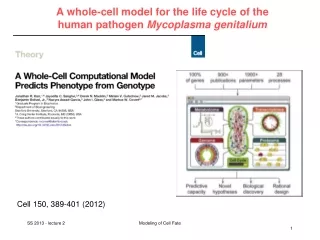
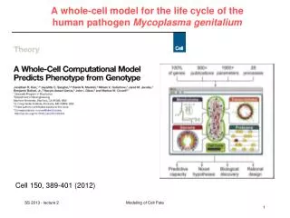
A whole-cell model for the life cycle of the human pathogen Mycoplasma genitalium. Cell 150, 389-401 (2012). Main aims. Describe the life cycle of a single cell from the level of individual molecules and their interactions

E N D
A whole-cell model for the life cycle of the human pathogen Mycoplasma genitalium Cell 150, 389-401 (2012) Modeling of Cell Fate
Main aims • Describethelifecycleof a singlecellfromthelevelof individual moleculesandtheirinteractions • Account forthespecificfunctionofeveryannotatedgeneproduct • accuratelypredict a widerangeof observable cellularbehaviors Problem: In a cell, everythingseemsconnectedtoeverything. Modeling of Cell Fate
Divide and conquer approach (Caesar):split whole-cell model into 28 independent submodels 28 submodels are built / parametrized / iterated independently Modeling of Cell Fate
Cell variables • System stateisdescribedby 16 cell variables • Coloredlines: cell variables affectedby individual submodels • Mathematicaltools: • Differential equations • Stochasticsimulations • Fluxbalanceanalysis Modeling of Cell Fate
Whole-cell model architecture Show movie. Q: Can treatment as independent processes lead to problems? Modeling of Cell Fate
Time step in molecular atomistic dynamics simulations • Toolong time stepleadstonumericalinstabilities • -> atomsmove „toofar“ alongthedirectionofattraction • Similarproblemsmayarise in whole-cellsimulation. • particlesofone type accumulate Modeling of Cell Fate
Whole-cell dynamic simulation algorithm Modeling of Cell Fate
Algo to identify initial conditions Modeling of Cell Fate
Initialize cell state Modeling of Cell Fate
Nucleotide states This state represents the polymerization, winding, modification, and protein occupancy of each nucleotide of each strand of each copy of the M. genitalium chromosome, and the (de)catenation status of the two sister chromosomes following replication. Modeling of Cell Fate
Protein Monomers are the direct result of successful translation events. Upon Translation, a monomer undergoes various steps towards maturation including deformylation, translocation, folding, and phosphorylation. A monomer can exist in many forms (nascent, processed (I), translocated, processed (II),folded, and mature) as it moves through the maturation pipeline. Modeling of Cell Fate
Ribosome Ribosomes are large ribonucleoproteins which synthesize polypeptides. The M. genitalium 70S ribosome is composed of two subunits – the 30S and 50S ribosomal subunits – which assemble on mRNA with assistance from initiation factors 1-3 (MG173, MG142, MG196). The 30S subunit is composed of 1 RNA and 20 protein monomer subunits. The 50S subunit is composed of 2 RNA and 32 protein monomer subunits. The 30S and 50S ribosomal subunits are believed to assemble in stereotyped patterns, and six GTPases – EngA, EngB, Era, Obg, RbfA, and RbgA – have been associated with ribosomal subunit assembly. The exact functions of the six GTPases are unknown. Modeling of Cell Fate
Ribosome Modeling of Cell Fate
Basic outline of the direct method of Gillespie (Step i) generate a list of the components/species and define the initial distribution at time t = 0. (Step ii) generate a list of possible events Ei (chemical reactions as well as physical processes). (Step iii) using the current component/species distribution, prepare a probability table P(Ei) of all the events that can take place. Compute the total probability P(Ei) : probability of event Ei. (Step iv) Pick two random numbers r1 and r2 [0...1] to decide which event E will occur next and the amount of time by which E occurs later since the most recent event. Resat et al., J.Phys.Chem. B 105, 11026 (2001) Bioinformatics III
Basic outline of the direct method of Gillespie Using the random number r1 and the probability table, the event E is determined by finding the event that satisfies the relation The second random number r2 is used to obtain the amount of time between the reactions As the total probability of the events changes in time, the time step between occurring steps varies. Steps (iii) and (iv) are repeated at each step of the simulation. The necessary number of runs depends on the inherent noise of the system and on the desired statistical accuracy. Resat et al., J.Phys.Chem. B 105, 11026 (2001) Bioinformatics III
Transcriptional regulation Modeling of Cell Fate
microarray expression analysis Modeling of Cell Fate
DNA repair simulation Modeling of Cell Fate
Non-coding RNA cleavage Modeling of Cell Fate
Model FtsZ polymerization Cell division in many bacterial species requires the assembly of an FtsZ ring at the cell membrane around the midplane of the cell. FtsZ is a homologue of eukaryotic tubulin that assembles into long polymers. These polymers are typically localized to the center of the cell, forming a membrane-bound ring. FtsZ is a GTPase, and GTP hydrolysis to GDP causes the FtsZ filaments to bend. This bending serves as one of the forces enabling cell division. Modeling of Cell Fate
Model FtsZ polymerization FtsZ can exist in one of multiple states: inactivated monomer, activated monomer (GTP bound), nucleated (dimer of two activated FtsZ molecules), elongated polymer of three or more GTP bound FtsZ molecules. Modeling of Cell Fate
Formation of macromolecular complexes The relative formation rate, riof each complex, i, is described by mass-action kinetics, m j : copy number of gene product j, V is the cell volume, sij : stoichiometry of subunit j in complex i. Modeling of Cell Fate
Model small-molecule metabolism by FBA Modeling of Cell Fate
V15 Flux Balance Analysis – Extreme Pathways Stoichiometric matrix S: m × n matrix with stochiometries of the n reactions as columns and participations of m metabolites as rows. The stochiometric matrix is an important part of the in silico model. With the matrix, the methods of extreme pathway and elementary mode analyses can be used to generate a unique set of pathways P1, P2, and P3 that allow to express all steady-state fluxes as linear combinations of P1 – P3. Papin et al. TIBS 28, 250 (2003) Bioinformatics III
Flux balancing Any chemical reaction requiresmass conservation. Therefore one may analyze metabolic systems by requiring mass conservation. Only required: knowledge about stoichiometry of metabolic pathways. For each metabolite Xi : dXi /dt = Vsynthesized – Vused + Vtransported_in – Vtransported_out Under steady-state conditions, the mass balance constraints in a metabolic network can be represented mathematically by the matrix equation: S· v = 0 where the matrix S is the stoichiometric matrix and the vector v represents all fluxes in the metabolic network, including the internal fluxes, transport fluxes and the growth flux. Bioinformatics III
Flux balance analysis Since the number of metabolites is generally smaller than the number of reactions (m < n) the flux-balance equation is typically underdetermined. Therefore there are generally multiple feasible flux distributions that satisfy the mass balance constraints. The set of solutions are confined to the nullspace of matrix S. S . v = 0 Bioinformatics III
Feasible solution set for a metabolic reaction network The steady-state operation of the metabolic network is restricted to the region within a pointed cone, defined as the feasible set. The feasible set contains all flux vectors that satisfy the physicochemical constrains. Thus, the feasible set defines the capabilities of the metabolic network. All feasible metabolic flux distributions lie within the feasible set. Edwards & Palsson PNAS 97, 5528 (2000) Bioinformatics III
True biological flux To find the „true“ biological flux in cells ( e.g. Heinzle, UdS) one needs additional (experimental) information, or one may impose constraints on the magnitude of each individual metabolic flux. The intersection of the nullspace and the region defined by those linear inequalities defines a region in flux space = the feasible set of fluxes. In the limiting case, where all constraints on the metabolic network are known, such as the enzyme kinetics and gene regulation, the feasible set may be reduced to a single point. This single point must lie within the feasible set. Bioinformatics III
Metabolism FBA simulation • microarray expression analysis Modeling of Cell Fate
DNA replication • microarray expression analysis Modeling of Cell Fate
DNA replication DNA naturally exists at a certain level of helicity, and this level of helical density is important for the DNA’s stability, its ability to fit in the cell, and its ability to bind proteins. M. genitalium has 3 topoisomerase proteins: DNA gyrase, topoisomerase I, and topoisomerase IV. These proteins transiently break a DNA strand to wind (topoisomerase I) or unwind (topoisomerase IV, gyrase) the DNA. Modeling of Cell Fate
Which states are affected by replication? Upon replication initiation (the binding of 29 DnaA-ATP molecules near the oriC by the Replication Initiation process class), the Replication process class tracks the progression of the replication proteins on the known chromosome sequences. Modeling of Cell Fate
Results from simulations Modeling of Cell Fate
Growth of virtual cell culture Growth of three cultures (dilutions indicated by shade of blue) and a blank control measured by OD550 of the pH indicator phenol red. The doubling time, t, was calculated using the equation at the top left from the additional time required by more dilute cultures to reach the same OD550 (black lines). The model calculations were consistent with the observed doubling time! Modeling of Cell Fate
Individual simulations Predicted growth dynamics of one life cycle of a population of 64 in silico cells Q: what is the source of the variability of the length of the cell cycle? (later) Modeling of Cell Fate
Chemical composition Comparison of the predicted and experimentally observed cellular chemical compositions Model calculations were consistent with the observed cellular chemical composition! Modeling of Cell Fate
Increase of cell mass Temporal dynamics of the total cell mass and four cell mass fractions of a representative in silico cell. Model calculations were consistent with the observed replication of major cell mass fractions. Modeling of Cell Fate
Metabolic flux rates Average predicted metabolic fluxes (from FBA modeling). Arrow brightness indicates flux magnitude. In agreement with exp data, the model predicts that the flux through glycolysis is >100-fold more than that through the pentose phosphate and lipid biosynthesis pathways. Modeling of Cell Fate
Metabolite concentrations Ratios of observed and average predicted concentrations of 39 metabolites. The predicted metabolite concentrations are within an order of magnitude of concentrations measured in Escherichia coli for 100% of the metabolites in one compilation of data and for 70% in a more recent high-throughput study. Modeling of Cell Fate
mRNA and protein synthesis events Temporal dynamics of cytadherence high-molecular-weight protein 2 (HMW2, MG218) mRNA and protein expression of one in silico cell. Red dashed lines indicate the direct link between mRNA synthesis and subsequent bursts in protein synthesis. Due to (a) the local effect of intermittent messenger RNA (mRNA) expression and (b) the global effect of stochastic protein degradation on the availability of free amino acids for translation, model predicts ‘‘burst-like’’ protein synthesis. This is comparable to exp. observations! Modeling of Cell Fate
Density of DNA-bound proteins Average density of all DNA-bound proteins and of the replication initiation protein DnaA and DNA and RNA polymerase of a population of 128 in silico cells. Top magnification : average density of DnaA at several sites near the oriC; DnaA forms a large multimeric complex at the sites indicated with asterisks, recruiting DNA polymerase to the oriC to initiate replication. Bottom left : location of the highly expressed rRNA genes.. Consistent with recent experimental data, the predicted high-occupancy RNA polymerase regions correspond to highly transcribed rRNAs and tRNAs. In contrast, the predicted DNA polymerase chromosomal occupancy is significantly lower and biased toward the terC. Modeling of Cell Fate
Exploration of genome Percentage of the chromosome that is predicted to have been bound (B) as functions of time. SMC is an abbreviation for the name of the chromosome partition protein (MG298). The model further predicts that the chromosome is explored very rapidly, with 50% of the chromosome having been bound by at least one protein within the first 6 min of the cell cycle and 90% within the first 20 min Modeling of Cell Fate
Dynamics of genome expression Percentage of the number of genes that are predicted to have been expressed (C) as functions of time. RNA polymerase contributes the most to chromosomal exploration, It binds 90% of the chromosome within the first 49 min of the cell cycle. On average, this results in expression of 90% of genes within the first 143 min. Modeling of Cell Fate
DNA-binding and dissociation dynamics DNA-binding and dissociation dynamics of the oriC DnaA complex (red) and of RNA (blue) and DNA (green) polymerases for one in silico cell. The oriC DnaA complex recruits DNA polymerase to the oriC to initiate replication, which in turn dissolves the oriC DnaA complex. RNA polymerase traces (blue line segments) indicate individual transcription events. The height, length, and slope of each trace represent the transcript length, transcription duration, and transcript elongation rate, respectively. Inset : several predicted collisions between DNA and RNA polymerases that lead to the displacement of RNA polymerases and incomplete transcripts. Modeling of Cell Fate
Predictions for cell-cycle regulation Distributions of the duration of three cell-cycle phases, as well as that of the total cell-cycle length, across 128 simulations. • There was relatively more cell-to-cell variation in the durations of the replication • initiation (64.3%) and replication (38.5%) stages than in cytokinesis (4.4%) or the overall cell cycle (9.4%). • This data raised two questions: • what is the source of duration variability in the initiation and replication phases; and • (2) why is the overall cell-cycle duration less varied than either of these phases? Modeling of Cell Fate
Replication initiation Replication initiation occurs as DnaA protein monomers bind or unbind stochastically and cooperatively to form a multimeric complex at the replication origin. When the complex is complete, DNA polymerase gains access to the origin, and the complex is displaced. Modeling of Cell Fate
Dynamics of macromolecule abundance Top : the size of the DnaA complex assembling at the oriC (in monomers of DnaA); middle, the copy number of the chromosome; Bottom : cytosolic dNTP concentration. The quantities of these macromolecules correlate strongly with the timing of key cell-cycle stages. Modeling of Cell Fate
What determines replication duration? We found a correlation (R2 = 0.49) between the predicted duration of replication initiation and the initial number of free DnaA monomers. The duration of the replication phase in individual cells is more closely related to the free dNTP content at the start of replication than to the dNTP content at the start of the cell cycle The durations of the initiation and replication phases are inversely related to each other in single cells. Cells that require extra time to initiate replication also build up a large dNTP surplus, leading to faster replication. Modeling of Cell Fate