Download
1 / 18
180 likes | 363 Views
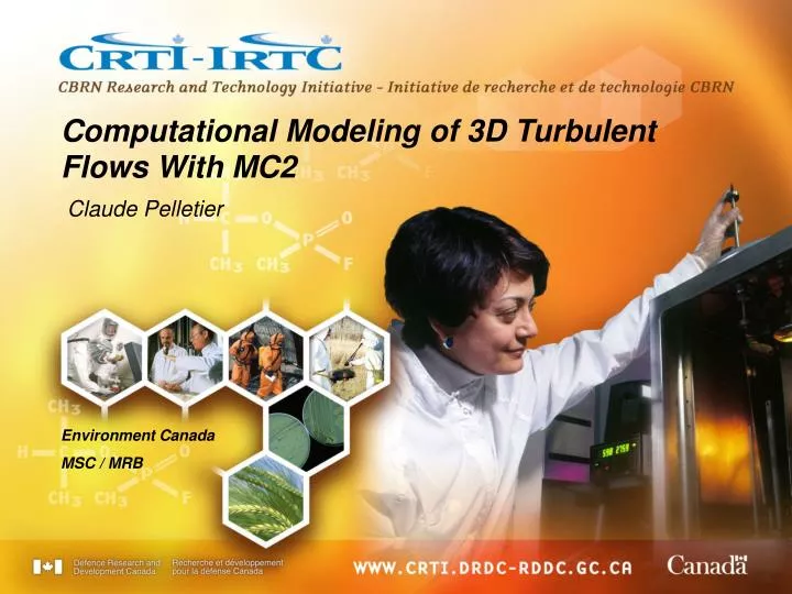
Computational Modeling of 3D Turbulent Flows With MC2. Claude Pelletier. Environment Canada MSC / MRB. Implementing 3D Turbulence for CRTI. Current public release of MC2 uses 1D turbulence (Z-axis) only

E N D
Computational Modeling of 3D Turbulent Flows With MC2 Claude Pelletier Environment Canada MSC / MRB
Implementing 3D Turbulence for CRTI • Current public release of MC2 uses 1D turbulence (Z-axis) only • Must implement XY contributions in order to increase grid resolution and move MC2 toward LES • Introduced in MC2 the Reynolds time-averaged form of the compressible Navier-Stokes equations + generalized 3D budget TKE equation • The resulting momentum equations are identical to filtered LES equation set when using a classic square box filter • Introduced TEB and latest RPN physics package (v. 4.3, to be released)
Turbulent momentum transport equations in Cartesian coordinates • Included all XY components of the dynamic Reynolds stress tensor • Added TKE gradient terms • Horizontal corrections introduced in all remaining transport equations • Modified operator splitting technique used by TKE solver • Finite difference discretization on Arakawa-C grid
MC2 Charney-Phillips vertical staggering Momentum levels (TKE, diffusion coeff.) Thermodynamic levels (T, q, gz, density)
6-level cascade computational setup Step 1: 2003/07/16 0:00 to 2003/07/17 9:00 CDT, ∆t=120 sec [∆x, ∆y]=50 km, 31 z levels [0 – 25000 ft] with 13 in PBL Z (m)
Step 2: 2003/07/16 5:00h to 2003/07/17 9:00 CDT, ∆t=30 sec [∆x, ∆y]=10 km, 45 z levels [0 – 25000 ft] with 13 in PBL Z (m)
Step 3: 2003/07/16 7:00 to 2003/07/17 9:00 CDT, ∆t=10 sec [∆x, ∆y]=2.5 km, 60 z levels [0 – 25000 ft] with 13 in PBL Z (m)
Step 4: 2003/07/16 9:00 to 2003/07/17 9:00 CDT, ∆t=5 sec [∆x, ∆y]=1 km, 60 z levels [0 - 25000 ft] with 13 in PBL Z (m)
Step 5: 2003/07/16 11:00 to 2003/07/17 9:00 CDT, ∆t = 5 sec [∆x, ∆y]=200 m, 60 z levels [0 - 25000 ft] with 13 levels in PBL Z (m)
Step 6: 2003/07/16, 14:00 – 18:00 CDT, 40 m mesh size, ∆t=1 sec 80 z levels with top sponge layer at 9500 ft Z (m) 1 sec of animation = 10 min of real time
Ratio of H/V motion components (OKC 16:00 CDT, 200 m mesh) Z = 1500 m Z = 2500 m >10
Ratio of H/V motion components (OKC 16:00 CDT, 40 m mesh size) Z = 1500 m Z = 2500 m >10
1D vs. 3D TKE profiles (OKC 16:00 CDT) 40 m 200 m
Vertical heat flux: resolved and subgrid scales (OKC 16:00 CDT) 40 m 200 m
Vertical heat flux: published LES results • 30 m resolution • SB1 and SB2: strong shear + moderate convection Moeng et al., J. Atmos.,Sci., 1994
With TEB: 2003/07/16 4:00 – 2003/07/17 4:00 CDT, 1 km mesh size, z = 25m TKE Potential temperature
Computational cost • 128-cpu runs on IBM supercomputer • 3D CFL number ≈ 0.5 • 3D terms account for ≈ 15% increase in CPU time at low to moderate resolutions • 3-fold increase in number of solver iterations at high resolution • Time step length is about the same for 1D and 3D computations at very high resolutions • Semi-Lagrangian transport allows reasonable time step even at high resolution