
Logistic Regression for Classification Methods
E N D
Presentation Transcript
STT592-002: Intro. to Statistical Learning Classification Methods Chapter 04 (part 01) Disclaimer: This PPT is modified based on IOM 530: Intro. to Statistical Learning "Some of the figures in this presentation are taken from "An Introduction to Statistical Learning, with applications in R" (Springer, 2013) with permission from the authors: G. James, D. Witten, T. Hastie and R. Tibshirani "
STT592-002: Intro. to Statistical Learning Outline: Response Var. is qualitative • Recall: • Chap3: Response var. Y is quantitative/numerical. • Chap3: what to do with categorical predictor X? • Chap4: Response var. Y is qualitative/categorical (eg: gender). classification.
STT592-002: Intro. to Statistical Learning Logistic Regression Overview: Classification methods Chap4: Logistic regression; LDA/QDA; KNN Chap7: Generalized Additive Models Chap8: Trees, Random Forest, Boosting Chap9: Support Vector Machines (SVM)
STT592-002: Intro. to Statistical Learning Outline: Response Var. is qualitative • Cases: • Orange Juice Brand Preference • Credit Card Default Data • Why Not Linear Regression? • Simple Logistic Regression • Logistic Function • Interpreting the coefficients • Making Predictions • Adding Qualitative Predictors • Multiple Logistic Regression
STT592-002: Intro. to Statistical Learning Case 1: OJ data (introduced briefly) library(MASS); library(ISLR) data(OJ); head(OJ) ? OJ ## to find more details about data OJ.
STT592-002: Intro. to Statistical Learning Case 1: Brand Preference for Orange Juice • We would like to predict what customers prefer to buy: Citrus Hill (CH) or Minute Maid (MM) orange juice? • The Y (Purchase) variable is categorical: 0 or 1 • The X (LoyalCH) variable is a numerical value (b/w 0 & 1) which specifies how much customers are loyal to Citrus Hill (CH) orange juice • Can we use Linear Regression when Y is categorical?
0.9 0.7 0.5 0.4 0.2 0.0 .0 .1 .2 .3 .4 .5 .6 .7 .8 .9 1.0 LoyalCH STT592-002: Intro. to Statistical Learning Why not Linear Regression? • When Y only takes on values of 0 and 1, why standard linear regression in inappropriate? • First need to consider ordering of Purchase 01. In practice, no particular reason that this needs to be the case. Purchase How do we interpret values greater than 1? How do we interpret values of Y below 0?
STT592-002: Intro. to Statistical Learning Problems • The regression line 0+1X can take on any value between negative and positive infinity • In the orange juice classification problem, Y can only take on two possible values: 0 or 1. • Therefore regression line almost always predicts wrong value for Y in classification problems
STT592-002: Intro. to Statistical Learning Solution: Use Logistic Function • Instead of trying to predict Y, let’s try to predict P(Y = 1), i.e., prob. a customer buys Citrus Hill (CH) juice. • Thus, we can model P(Y = 1) using a function that gives outputs between 0 and 1. • We can use Logistic Regression! X is centerized
STT592-002: Intro. to Statistical Learning Logistic Regression Model
1 CH 0.75 0.5 MM 0.25 .0 .2 .4 .6 .7 .9 0 LoyalCH STT592-002: Intro. to Statistical Learning Logistic Regression • Logistic regression is very similar to linear regression • We come up with b0 and b1 to estimate 0 and 1. • We have similar problems and questions as in linear regression • e.g. Is 1 equal to 0? • How sure are we about our guesses for 0 and 1? P(Purchase) If LoyalCH is about .6 then Pr(CH) .7.
STT592-002: Intro. to Statistical Learning Case 2: Credit Card Default Data • To predict customers that are likely to default • Possible X variables are: • Annual Income • Monthly credit card balance • The Y variable (Default) is categorical: Yes or No • How do we check the relationship between Y and X?
STT592-002: Intro. to Statistical Learning The Default Dataset library(MASS); library(ISLR) data(Default) head(Default)
STT592-002: Intro. to Statistical Learning Case 2: Default Dataset (Fig 4.1)
STT592-002: Intro. to Statistical Learning Default Dataset: replicate Fig 4.1 library(MASS); library(ISLR) data(Default); ; head(Default); attach(Default) plot(balance[default=="Yes"], income[default=="Yes"], pch="+", col="darkorange") points(balance[default=="No"], income[default=="No"], pch=21, col="lightblue")
STT592-002: Intro. to Statistical Learning Default Dataset: replicate Fig 4.1 library(MASS); library(ISLR) data(Default); head(Default); attach(Default) par(mfrow=c(1,2)) plot(default, balance, col=c("lightblue", "darkorange"), xlab="Default", ylab="Balance") plot(default, income, col=c("lightblue", "darkorange"), xlab="Default", ylab="Income")
STT592-002: Intro. to Statistical Learning Default Dataset: Be careful if you switch the order… library(MASS); library(ISLR) data(Default); head(Default); attach(Default) par(mfrow=c(1,2)) plot(balance, default, col=c("lightblue", "darkorange"), xlab="Default", ylab="Balance") plot(income, default, col=c("lightblue", "darkorange"), xlab="Default", ylab="Income")
STT592-002: Intro. to Statistical Learning Review: Why not Linear Regression? • If we fit a linear regression to the Default data, • then for very low balances we predict a negative probability, • and for high balances we predict a probability above 1! When Balance < 500, Pr(default) is negative!
STT592-002: Intro. to Statistical Learning Logistic Function on Default Data • Now probability of default is close to, but not less than zero for low balances. • Close to but not above 1 for high balances
STT592-002: Intro. to Statistical Learning Case 2: Default Dataset: library(MASS); library(ISLR) attach(Default); head(Default) # Logistic Regression glm.fit=glm(default~balance,family=binomial) summary(glm.fit)
STT592-002: Intro. to Statistical Learning The Default Dataset: Extra note library(MASS); library(ISLR); attach(Default); head(Default) glm.fit=glm(default~balance,family=binomial) summary(glm.fit) with(glm.fit, null.deviance - deviance) with(glm.fit, df.null - df.residual) with(glm.fit, pchisq(null.deviance - deviance, df.null - df.residual, lower.tail = FALSE)) logLik(glm.fit) Suppose that we have a statistical model of some data. Let L be the maximum value of the likelihood function for the model; let k be the number of estimated parameters in the model. Then the AIC value of the model is the following. Given a set of candidate models for the data, the preferred model is the one with the minimum AIC value
STT592-002: Intro. to Statistical Learning Interpreting 1 • We see that β1-hat = 0.0055; • this indicates that an increase in balance is associated with an increase in prob. of default. • To be precise, a one-unit increase in balance is associated with an increase in the log odds of default by 0.0055 units.
STT592-002: Intro. to Statistical Learning Interpreting 1 • We see that β1-hat = 0.0055; • this indicates that an increase in balance is associated with an increase in prob. of default. • To be precise, a one-unit increase in balance is associated with an increase in the log odds of default by 0.0055 units.
STT592-002: Intro. to Statistical Learning Interpreting 1 • Interpreting what 1means is not very easy with logistic regression, simply because we are predicting P(Y) and not Y. • If 1=0, this means there is no relationship b/w Pr(Y|X) & X. • For logistic regression, increasing X by one unit changes the log odds by 1. • If 1 >0, this means that when X gets larger so does the probability that Y = 1. • If 1<0, this means that when X gets larger, the probability that Y = 1 gets smaller. • But how much bigger or smaller depends on where we are on the slope?
STT592-002: Intro. to Statistical Learning Are coefficients significant? • To perform a hypothesis test to see whether we can be sure that are 0 and 1significantly different from zero. • Use a Z test instead of a T test, but of course that doesn’t change the way we interpret p-value. • Here p-value for balance is very small, and b1 is positive, so we are sure that if balance increase, then probability of default will increase as well. Why Z-test statistics: (1) https://stats.stackexchange.com/questions/60074/wald-test-for-logistic-regression (2) https://www.quora.com/In-Stata-and-R-output-why-is-z-test-other-than-t-test-used-in-logistic-regression-to-assess-the-significance-of-the-individual-variables
STT592-002: Intro. to Statistical Learning Making Prediction • Suppose an individual has an average balance of X=$1000. What is their prob. of default? • Predicted probability of default for an individual with a balance of $1000 is less than 1%. • For a balance of $2000, probability is much higher, and equals to 0.586 (58.6%).
STT592-002: Intro. to Statistical Learning Logistics Regression for Default Dataset: library(MASS); library(ISLR) attach(Default); head(Default) # Logistic Regression glm.fit=glm(default~student,family=binomial) summary(glm.fit)$coef The estimated intercept is typically not of interest. Its main purpose is to adjust the average fitted prob to the proportion of ones in the data.
STT592-002: Intro. to Statistical Learning Qualitative Predictors in Logistic Regression • We can predict if an individual default by checking if she is a student or not. Thus we can use a qualitative variable “Student” coded as (Student = 1, Non-student =0). • b1 is positive: This indicates students tend to have higher default probabilities than non-students
STT592-002: Intro. to Statistical Learning Multiple Logistic Regression • We can fit multiple logistic just like regular regression
STT592-002: Intro. to Statistical Learning Example: Default Dataset for multiple logistic regression # Logistic Regression on student, balance and income glm.fit=glm(default~student+balance+income,family=binomial) summary(glm.fit) coef(glm.fit) summary(glm.fit)$coef
STT592-002: Intro. to Statistical Learning Multiple Logistic Regression- Default Data • Predict Default using: • Balance (quantitative) • Income (quantitative) • Student (qualitative)
STT592-002: Intro. to Statistical Learning Predictions • A student with a credit card balance of $1,500 and an income of $40,000 has an estimated probability of default
STT592-002: Intro. to Statistical Learning An Apparent Contradiction! Positive Negative
STT592-002: Intro. to Statistical Learning Students (Orange) vs. Non-students (Blue) The left panel provides a graphical illustration of this apparent paradox. The orange and blue solidlines show average default rates for students and non-students, respectively, as a function of credit card balance. Negative coefficient for student in multiple logistic regression indicates that for a fixed value of balance and income, a student is less likely to default than a non-student…
STT592-002: Intro. to Statistical Learning Summary: To whom should credit be offered? • A student is risker than non students if no information about credit card balance is available • However, that student is less risky than a non student with same credit card balance!
STT592-002: Intro. to Statistical Learning Logistic regression with more than 2 response classes • 2-class Logistic regression model can be extended to multiple-class cases in different ways. • In practice they tend not to be used all that often. • Instead discriminant analysis (next section) is popular for multiple-class classification.