Download
1 / 10
100 likes | 415 Views
Economic Growth with Technological Progress. Introduction. The Solow growth model as developed in Chapter 8 showed how changes in the capital stock and population growth affect the long-run level of output of the economy.

E N D
Introduction • The Solow growth model as developed in Chapter 8 showed how changes in the capital stock and population growth affect the long-run level of output of the economy. • The last part of Chapter 8 adds changes in technology to complete the model. • The complete Solow growth model can then be used to examine how public policies influence saving and investment and thus affect long-run economic growth.
Introduction (cont’d) • While the Solow model is a useful tool for understanding economic growth, it is not without its weaknesses. Macroeconomists have attempted to address some of these weaknesses to better understand the process of economic growth.
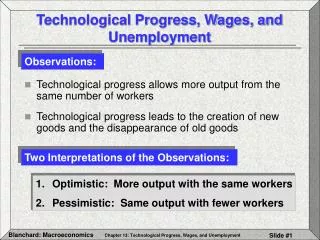
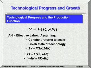
Technological Progress in the Solow Model • The Solow model provided an explanation of persistently rising output, but we have not yet explained rising living standards. To do so, we incorporate technological progress, meaning that we are able to produce more output with a given amount of capital and labor.
New Production Function • In general, technological progress can take many different forms. By far the easiest form to analyze is labor-augmenting technological progress. • We write the production function as: Y=F(K,EL) • The new variable, E, represents the efficiency of labor, which depends on the skills and education of the workforce. • The idea is that a more skilled and better trained workforce can produce more output with a given capital stock. • As an example, think of capital as consisting of personal computers and labor efficiency as being knowledge of software packages.
We represent technological progress as an exogenous increase in the value of E through time. That is, we suppose that E grows at the rate g. • Over time, even if K and L are constant, each worker will be able to produce more and more output. • For example, a 2 percent improvement in the efficiency of labor means that 98 workers can now do a job that used to require 100 workers. • The product EL measures effective workers.
The key to the analysis in this case is that changes in labor efficiency act exactly like changes in population. • Just from looking at the production function, it is evident that changes in E most affect output in just the same way that changes in L affect output. • If we have 2-percent population growth and no technological progress, then ELgrows at 2 percent • Likewise, if we have no population growth and 2-percent technological progress, then ELgrows at 2 percent.
Suppose, therefore, that population growth is zero and technological progress is at the rate g. • By following the same reasoning used in the case of population growth, we see that K must grow at the rate g in steady state. Output also grows at the rate g. • In this steady state, capital per effective worker — K/ EL— is constant. • The only difference from the previous analysis is that the actual capital-labor ratio, K/L, now grows through time at the rate g, implying in turn that output per person now grows at the rate g. Thus, this model can finally explain rising living standards.
Putting the Pieces Together • We can now summarize the Solow model when all three sources of growth – changes in capital, changes in labor, and changes in technology (labor efficiency) – are present.
Suppose that the population is growing at the rate n (say, 1 percent per year), and the efficiency of labor is growing at the rate g (say, 2 percent per year). Then effective workers are growing at the (n+g) rate , which equals 3 percent per year. • Since capital per efficiency unit of labor is constant in steady state, it follows that the capital stock must also be growing at 3 percent per year. Consequently, total output will be growing at 3 percent per year. • Although capital per effective worker is constant, capital per person (the capital-labor ratio) is growing at 2 percent per year. Similarly, output per person and consumption per person are also growing at 2 percent per year in this steady state.