Download
1 / 66
670 likes | 922 Views
AMS 572 Group Project. Simple Linear Regression & Correlation Instructor: Prof. Wei Zhu 11/21/2013. Outline. Motivation & Introduction – Lizhou Nie A Probabilistic Model for Simple Linear Regression – Long Wang Fitting the Simple Linear Regression Model – Zexi Han

E N D
AMS 572 Group Project • Simple Linear Regression & Correlation • Instructor: Prof. Wei Zhu • 11/21/2013
Outline • Motivation & Introduction – Lizhou Nie • A Probabilistic Model for Simple Linear Regression – Long Wang • Fitting the Simple Linear Regression Model – Zexi Han • Statistical Inference for Simple Linear Regression – Lichao Su • Regression Diagnostics – Jue Huang • Correlation Analysis – Ting Sun • Implementation in SAS – Qianyi Chen • Application and Summary – JieShuai
1. Motivation Fig. 1.2 Obama & Romney during Presidential Election Campaign http://outfront.blogs.cnn.com/2012/08/14/the-most-negative-in-campaign-history/ Fig. 1.1 Simplified Model for Solar System http://popperfont.net/2012/11/13/the-ultimate-solar-system-animated-gif/
Introduction • Regression Analysis • Linear Regression: • Simple Linear Regression: {y, x} • Multiple Linear Regression: {y; x1, … , xp} • Multivariate Linear Regression: {y1, … , yn; x1, … , xp} • Correlation Analysis • Pearson Product-Moment Correlation Coefficient: Measurement of Linear Relationship between Two Variables
History • Adrien-Marie Legendre • Earliest Form of • Regression: Least • Square Method • George UdnyYule • & Karl Pearson • Extention to a • More Generalized • Statistical Context • Carl Friedrich Gauss • Further Development of • Least Square Theory • including Gauss-Markov • Theorem • Sir Francis Galton • Coining the Term “Regression” http://en.wikipedia.org/wiki/Regression_analysis http://en.wikipedia.org/wiki/Adrien_Marie_Legendre http://en.wikipedia.org/wiki/Carl_Friedrich_Gauss http://en.wikipedia.org/wiki/Francis_Galton http://www.york.ac.uk/depts/maths/histstat/people/yule.gif http://en.wikipedia.org/wiki/Karl_Pearson
2. A Probabilistic Model • Simple Linear Regression • - Special Case of Linear Regression • - One Response Variable to One Explanatory Variable • General Setting • -We Denote Explanatory Variableas Xi’s and Response Variable as Yi’s • - N Pairs of Observations {xi, yi}, i = 1 to n
2. A Probabilistic Model • Sketch the Graph (29, 5.5)
2. A Probabilistic Model • In Simple Linear Regression, Data is described as: • Where ~ N(0, ) • The Fitted Model: • Where - Intercept • - Slope of Regression Line
3. Fitting the Simple Linear Regression Model Table 3.1. Fig 3.1. Scatter plot of tire tread wear vs. mileage. From: Statistics and Data Analysis; Tamhane and Dunlop; Prentice Hall.
3. Fitting the Simple Linear Regression Model The difference between the fitted line and real data is is the vertical distance between fitted line and the real data Our goal: minimize the sum of square Fig 3.2.
3. Fitting the Simple Linear Regression Model LeastSquareMethod
3. Fitting the Simple Linear Regression Model Tosimplify,wedenote:
3. Fitting the Simple Linear Regression Model Backtotheexample:
3. Fitting the Simple Linear Regression Model • Therefore, the equation of fitted line is: Not enough!
3. Fitting the Simple Linear Regression Model • CheckthegoodnessoffitofLSline • We define: • Prove: • The ratio: • is called the coefficient of determination SST: total sum of squares SSR: Regression sum of squares SSE: Error sum of squares
3. Fitting the Simple Linear Regression Model • Check the goodness of fit of LS line • Back to the example: where the sign of r follows from the sign of since 95.3% of the variation in tread wear is accounted for by linear regression on mileage, the relationship between the two is strongly linear with a negative slope.
3. Fitting the Simple Linear Regression Model • r is the sample correlation coefficient between X and Y: • For the simple linear regression,
3. Fitting the Simple Linear Regression Model • Estimation of The variance measures the scatter of the around their means • An unbiased estimate of is given by
3. Fitting the Simple Linear Regression Model • From theexample, we have SSE=2351.3 and n-2=7,therefore • Which has 7d.f. The estimate of is
Under the normal error assumption * Point estimators: * Sampling distributions of and :
Derivation For mathematical derivations, please refer to the Tamhane and Dunlop text book, P331.
Statistical Inference on β0 and β1 * Pivotal Quantities (P.Q.’s): * Confidence Intervals (C.I.’s):
Hypothesis tests: . Reject at level if • A useful application is to show whether there is a linear relationship between x and y Reject at level if
Analysis of Variance (ANOVA) Mean Square: A sum of squares divided by its degrees of freedom.
Analysis of Variance (ANOVA) ANOVA Table
5. Regression Diagnostics • 5.1 Checking the Model Assumptions • 5.1.1 Checking for Linearity • 5.1.2 Checking for Constant Variance • 5.1.3 Checking for Normality • Primary tool: residual plots • 5.2 Checking for Outliers and Influential Observations • 5.2.1 Checking for Outliers • 5.2.2 Checking for Influential Observations • 5.2.3 How to Deal with Outliers and Influential Observations
5. Regression Diagnostics • 5.1 Checking the Model Assumptions • 5.1.1 Checking for Linearity • 5.1.2 Checking for Constant Variance • 5.1.3 Checking for Normality • Primary tool: residual plots • 5.2 Checking for Outliers and Influential Observations • 5.2.1 Checking for Outliers • 5.2.2 Checking for Influential Observations • 5.2.3 How to Deal with Outliers and Influential Observations
5. Regression Diagnostics • 5.1.1 Checking for Linearity • Table 5.1 The,,, for the Tire Wear Data • Figure 5.1 S,, for the Tire Wear Data
5. Regression Diagnostics • 5.1.1 Checking for Linearity (Data transformation) • Figure 5.2 Typical Scatter Plot Shapes and Corresponding Linearizing Transformations
5. Regression Diagnostics • 5.1.1 Checking for Linearity • (Data transformation) • Table 5.2 The,,,, for the Tire Wear Data • Figure 5.2 S,, for the Tire Wear Data
5. Regression Diagnostics • 5.1 Checking the Model Assumptions • 5.1.1 Checking for Linearity • 5.1.2 Checking for Constant Variance • 5.1.3 Checking for Normality • Primary tool: residual plots • 5.2 Checking for Outliers and Influential Observations • 5.2.1 Checking for Outliers • 5.2.2 Checking for Influential Observations • 5.2.3 How to Deal with Outliers and Influential Observations
5. Regression Diagnostics • 5.1.2 Checking for Constant Variance • Plot the residuals against the fitted value • If the constant variance assumption is correct, the dispersion of the ’s is approximately constant with respect to the ’s. • Figure 5.4 Plots of Residuals • Figure 5.3 Plots of Residuals
5. Regression Diagnostics • 5.1 Checking the Model Assumptions • 5.1.1 Checking for Linearity • 5.1.2 Checking for Constant Variance • 5.1.3 Checking for Normality • Primary tool: residual plots • 5.2 Checking for Outliers and Influential Observations • 5.2.1 Checking for Outliers • 5.2.2 Checking for Influential Observations • 5.2.3 How to Deal with Outliers and Influential Observations
5. Regression Diagnostics • 5.1.3 Checking for normality • Make a normal plot of the residuals • They have a zero mean and an approximately constant variance. • (assuming the other assumptions about the model are correct) • Figure 5.5 N
5. Regression Diagnostics • 5.1 Checking the Model Assumptions • 5.1.1 Checking for Linearity • 5.1.2 Checking for Constant Variance • 5.1.3 Checking for Normality • Primary tool: residual plots • 5.2 Checking for Outliers and Influential Observations • 5.2.1 Checking for Outliers • 5.2.2 Checking for Influential Observations • 5.2.3 How to Deal with Outliers and Influential Observations
5. Regression Diagnostics • Outlier: • an observation that does not follow the general pattern of the relationship between y and x. A large residual indicates an outlier. • Standardized residuals are given by • If , then the corresponding observation may be regarded as an outlier. • Influential Observation: • an influential observation has an extreme x-value, an extreme y-value, or both. • If we express the fitted value of y as a linear combination of all the • If , then the corresponding observations may be regarded as influential observation.
5. Regression Diagnostics • 5.2 Checking for Outliers and Influential Observations • Table 5.3 Standard residuals & leverage for transformed data
MATLAB Code for Regression Diagnostics • clear;clc; • x = [0 4 8 12 16 20 24 28 32]; • y = [394.33 329.50 291.00 255.17 229.33 204.83 179.00 163.83 150.33]; • y1 = log(y); %data transformation • p = polyfit(x,y,1) %linear regression predicts y from x • % p = polyfit(x,log(y),1) • yfit = polyval(p,x) %use p to predict y • yresid = y - yfit%compute the residuals • %yresid = y1 - exp(yfit) %residual for transformed data • ssresid = sum(yresid.^2); %residual sum of squares • sstotal = (length(y)-1) * var(y); %sstotal • rsq = 1 - ssresid/sstotal; %R square • normplot(yresid) %normal plot for residuals • [h,p,jbstat,critval]=jbtest(yresid) %test normality • scatter(x,y,500,'r','.') %generate the scatter plots • lsline • laxis([-5,35,-10,25]) • xlabel('x_i') • ylabel('y_i') • Title('plot of ...') • fori = 1:length(x) % check for outliers • p(i) = yresid(i)/std(yresid)/sqrt(1-1/length(x)-(yresid(i)-mean(yresid)^2)/(yresid(i)-mean(yresid))^2) • end • %check for influential observations • for j = 1:length(x) • q(i) = 1/length(x)+(x(i)-mean(x))^2/960 • end
6.1 Correlation Analysis • Why we need this? • Regression analysis is used to model the relationship between two variables. • But when there is no such distinction and both variables are random, correlation analysis is used to study the strength of the relationship.
6.1 Correlation Analysis- Example Example Flu reported Life expectancy Temperature People who get flu shot Economy level Economic growth Figure 6.1
6.2 Bivariate Normal Distribution • Because we need to investigate the correlation between X,Y • Source:http://wiki.stat.ucla.edu/socr/index.php/File:SOCR_BivariateNormal_JS_Activity_Fig7.png Figure 6.2
6.2 Why introduce Bivariate Normal Distribution? • First, we need to do some computation. • Compare with: • So, if (X,Y) have a bivariate normal distribution, then the regression model is true
6.3Statistical Inference of r • Define the r.v. R corresponding to r • But the distribution of R is quite complicated f(r) f(r) f(r) f(r) r r r -0.3 r -0.7 0 0.5 Figure 6.3
6.3 Exact testwhen ρ=0 • Test: H0 : ρ=0 , Ha : ρ≠0 • Test statistic: • Reject H0 iff • Example • A researcher wants to determine if two test instruments give similar results. The two test instruments are administered to a sample of 15 students. The correlation coefficient between the two sets of scores is found to be 0.7. Is this correlation statistically significant at the .01 level? • H0 : ρ=0 , Ha : ρ≠0 • 3.534 = t0 > t13, .005 = 3.012 • So, we reject H0
6.3Note:They are the same! • Because • So • We can say • H0: β1=0 are equivalent to H0: ρ=0
6.3Approximate test when ρ≠0 • Because that the exact distribution of R is not very useful for making inference on ρ, • R.A Fisher showed that we can do the following linear transformation, to let it be approximate normal distribution. • That is,
6.3Steps to do the approximate test on ρ • 1,H0 : ρ= ρ0 vs. H1 : ρ ≠ ρ0 • 2, point estimator • 3, T.S. • 4, C.I