Linear Modelling I
Linear Modelling I. Richard Mott Wellcome Trust Centre for Human Genetics. Synopsis. Linear Regression Correlation Analysis of Variance Principle of Least Squares. Correlation. Correlation and linear regression. Is there a relationship? How do we summarise it? Can we predict new obs ?


Linear Modelling I
E N D
Presentation Transcript
Linear Modelling I Richard Mott Wellcome Trust Centre for Human Genetics
Synopsis • Linear Regression • Correlation • Analysis of Variance • Principle of Least Squares
Correlation and linear regression • Is there a relationship? • How do we summarise it? • Can we predict new obs? • What about outliers?
Correlation Coefficient r • r=1 perfect positive linear • r=-1 perfect negative linear • -1 < r < 1 • r=0 no relationship • r=0.6
Calculation of r • Data
Correlation in R > cor(bioch$Biochem.Tot.Cholesterol,bioch$Biochem.HDL,use="complete") [1] 0.2577617 > cor.test(bioch$Biochem.Tot.Cholesterol,bioch$Biochem.HDL,use="complete") Pearson's product-moment correlation data: bioch$Biochem.Tot.Cholesterol and bioch$Biochem.HDL t = 11.1473, df = 1746, p-value < 2.2e-16 alternative hypothesis: true correlation is not equal to 0 95 percent confidence interval: 0.2134566 0.3010088 sample estimates: cor 0.2577617 > pt(11.1473,df=1746,lower.tail=FALSE) # T distribution on 1746 degrees of freedom [1] 3.154319e-28
Linear Regression Fit a straight line to data • a intercept • b slope • ei error • Normally distributed • E(ei) = 0 • Var(ei) = s2
Example: simulated data R code > # simulate 30 data points > x <- rnorm(30) > e <- rnorm(30) > x <- 1:30 > e <- rnorm(30,0,5) > y <- 1 + 3*x + e > # fit the linear model > f <- lm(y ~ x) > # plot the data and the predicted line > plot(x,y) > abline(reg=f) > print(f) Call: lm(formula = y ~ x) Coefficients: (Intercept) x -0.08634 3.04747
Least Squares • Estimate a, b by least squares • Minimise sum of squared residuals between y and the prediction a+bx • Minimise
Why least squares? • LS gives simple formulae for the estimates for a, b • If the errors are Normally distributed then the LS estimates are “optimal” In large samples the estimates converge to the true values No other estimates have smaller expected errors LS = maximum likelihood • Even if errors are not Normal, LS estimates are often useful
Analysis of Variance (ANOVA) LS estimates have an important property: they partition the sum of squares (SS) into fitted and error components • total SS = fitting SS + residual SS • only the LS estimates do this
ANOVA in R > anova(f) Analysis of Variance Table Response: y Df Sum Sq Mean Sq F value Pr(>F) x 1 20872.7 20872.7 965 < 2.2e-16 *** Residuals 28 605.6 21.6 > pf(965,1,28,lower.tail=FALSE) [1] 3.042279e-23
Hypothesis testing • no relationship between y and x • Assume errors ei are independent and normally distributed N(0,s2) • If H0 is true then the expected values of the sums of squares in the ANOVA are • degrees freedom • Expectation • F ratio = (fitting MS)/(residual MS) ~ 1 under H0 • F >> 1 implies we reject H0 • F is distributed as F(1,n-2)
Degrees of Freedom • Suppose are iid N(0,1) • Then ie n independent variables • What about ? • These values are constrained to sum to 0: • Therefore the sum is distributed as if it comprised one fewer observation, hence it has n-1 df (for example, its expectation is n-1) • In particular, if p parameters are estimated from a data set, then the residuals have p constraints on them, so they behave like n-p independent variables
The F distribution • If e1….en are independent and identically distributed (iid) random variables with distribution N(0,s2), then: • e12/s2 … en2/s2 are each iid chi-squared random variables with chi-squared distribution on 1 degree of freedom c12 • The sum Sn = Si ei2/s2 is distributed as chi-squared cn2 • If Tm is a similar sum distributed as chi-squared cm2, but independent of Sn, then (Sn/n)/(Tm/m) is distributed as an F random variable F(n,m) • Special cases: • F(1,m) is the same as the square of a T-distribution on m df • for large m, F(n,m) tends to cn2
ANOVA – HDL example HDL = 0.2308 + 0.4456*Cholesterol > ff <- lm(bioch$Biochem.HDL ~ bioch$Biochem.Tot.Cholesterol) > ff Call: lm(formula = bioch$Biochem.HDL ~ bioch$Biochem.Tot.Cholesterol) Coefficients: (Intercept) bioch$Biochem.Tot.Cholesterol 0.2308 0.4456 > anova(ff) Analysis of Variance Table Response: bioch$Biochem.HDL Df Sum Sq Mean Sq F value Pr(>F) bioch$Biochem.Tot.Cholesterol 1 149.660 149.660 1044 Residuals 1849 265.057 0.143 > pf(1044,1,28,lower.tail=FALSE) [1] 1.040709e-23
correlation and ANOVA • r2= FSS/TSS = fraction of variance explained by the model • r2 = F/(F+n-2) • correlation and ANOVA are equivalent • Test of r=0 is equivalent to test of b=0 • T statistic in R cor.test is the square root of the ANOVA F statistic • r does not tell anything about magnitudes of estimates of a, b • r is dimensionless
Effect of sample size Total Cholesterol vs HDL data Example R session to sample subsets of data and compute correlations seqq <- seq(10,300,5) corr <- matrix(0,nrow=length(seqq),ncol=2) colnames(corr) <- c( "sample size", "P-value") n <- 1 for(i in seqq) { res <- rep(0,100) for(j in 1:100) { s <- sample(idx,i) data <- bioch[s,] co <- cor.test(data$Biochem.Tot.Cholesterol, data$Biochem.HDL,na="pair") res[j] <- co$p.value } m <- exp(mean(log(res))) cat(i, m, "\n") corr[n,] <- c(i, m) n <- n+1 }
Calculating the right sample size n • The R library “pwr” contains functions to compute the sample size for many problems, including correlation pwr.r.test() and ANOVA pwr.anova.test()
Problems with non-linearityAll plots have r=0.8 (taken from Wikipedia)
Non-Parametric CorrelationSpearman Rank Correlation Coefficient • Replace observations by their ranks • eg x= ( 5, 1, 4, 7 ) -> rank(x) = (3,1,2,4) • Compute sum of squared differences between ranks • in R: • cor( x, y, method=“spearman”) • cor.test(x,y,method=“spearman”)
Spearman Correlation > cor.test(xx,y, method=“pearson”) Pearson's product-moment correlation data: xx and y t = 0.0221, df = 28, p-value = 0.9825 alternative hypothesis: true correlation is not equal to 0 95 percent confidence interval: -0.3566213 0.3639062 sample estimates: cor 0.004185729 > cor.test(xx,y,method="spearman") Spearman's rank correlation rho data: xx and y S = 2473.775, p-value = 0.01267 alternative hypothesis: true rho is not equal to 0 sample estimates: rho 0.4496607
Multiple Correlation • The R cor function can be used to compute pairwise correlations between many variables at once, producing a correlation matrix. • This is useful for example, when comparing expression of genes across subjects. • Gene coexpression networks are often based on the correlation matrix. • in R mat <- cor(df, na=“pair”) • computes the correlation between every pair of columns in df, removing missing values in a pairwise manner • Output is a square matrix correlation coefficients
One-Way ANOVA • Model y as a function of a categorical variable taking p values • eg subjects are classified into p families • want to estimate effect due to each family and test if these are different • want to estimate the fraction of variance explained by differences between families – ( an estimate of heritability)
One-Way ANOVA LS estimators average over group i
One-Way ANOVA • Variance is partitioned in to fitting and residual SS residual SS with groups n-p degrees of freedom total SS n-1 fitting SS between groups p-1
One-Way ANOVA Under Ho: no differences between groups F ~ F(p-1,n-p)
One-Way ANOVA in R fam <- lm( bioch$Biochem.HDL ~ bioch$Family ) > anova(fam) Analysis of Variance Table Response: bioch$Biochem.HDL Df Sum Sq Mean Sq F value Pr(>F) bioch$Family 173 6.3870 0.0369 3.4375 < 2.2e-16 *** Residuals 1727 18.5478 0.0107 --- Signif. codes: 0 '***' 0.001 '**' 0.01 '*' 0.05 '.' 0.1 ' ' 1 >
Non-ParametricOne-Way ANOVA • Kruskall-Wallis Test • Useful if data are highly non-Normal • Replace data by ranks • Compute average rank within each group • Compare averages • kruskal.test( formula, data )
Factors in R • Grouping variables in R are called factors • When a data frame is read with read.table() • a column is treated as numeric if all non-missing entries are numbers • a column is boolean if all non-missing entries are T or F (or TRUE or FALSE) • a column is treated as a factor otherwise • the levels of the factor is the set of distinct values • A column can be forced to be treated as a factor using the function as.factor(), or as a numeric vector using as.numeric()
Linear Modelling in R • The R function lm() fits linear models • It has two principal arguments (and some optional ones) • f <- lm( formula, data ) • formula is an R formula • data is the name of the data frame containing the data (can be omitted, if the variables in the formula include the data frame)
formulae in R • Biochem.HDL ~ Biochem$Tot.Cholesterol • linear regression of HDL on Cholesterol • 1 df • Biochem.HDL ~ Family • one-way analysis of variance of HDL on Family • 173 df • The degrees of freedom are the number of independent parameters to be estimated
ANOVA in R • f <- lm(Biochem.HDL ~ Tot.Cholesterol, data=biochem) • [OR f <- lm(biochem$Biochem.HDL ~ biochem$Tot.Cholesterol)] • a <- anova(f) • f <- lm(Biochem.HDL ~ Family, data=biochem) • a <- anova(f)
Contingency Tables • Data are a table of counts, with the row and column margins fixed. • Ho: the counts in each cell are consistent with the rows and columns acting independently