Download
1 / 48
490 likes | 515 Views
Explore the definition, representation, and operations of trees in computer science, including general principles, ways of thinking, and various applications like coding, parsing, and decision making. Learn about tree structures and different tree representations such as list, sibling, and array. Dive into the concepts of depth, height, and balancing of nodes in tree data structures. Discover how tree operations like copying, traversals, insertion, and deletion are performed efficiently.

E N D
TreesGeneral principlesWays of thinking Chapter 17 & 18 in DS&PS Chapter 4 in DS&AA
Applications • Coding • Huffman, prefix • Parsing/Compiling • tree is standard internal representation for code • Information Storage/Retrieval • binary trees, AA-trees, AVL, Red-Black, Splay • Game-Playing (Scenario analysis) • virtual trees • alpha-beta search • Decision Trees • representation of choices • automatically constructed from data
General Trees • Tree Definition • distinguished root node • all other node’s have unique, sole parent • Depth of a node: • number of edges from root to node • Height of a node: • number of edges from node to deepest descendant • Balanced: • Goal: O(log n) insert/delete/find • height of any sons of any node differs by less than 1 (k) • K-arity: • nodes have at most k sons
Depth of a Node 0 1 1 1 2 2 2 Often convenient to add another field to node structure for additional information such as: depth, height, visited, cost, father, number of visits, number of nodes below, etc.
Height of a Node 3 2 1 0 0 0 0 0 1 0 0
Simple Relationships • Leaf <=> height is 0 • Height of a node is 1+maximum height of sons • Root <=> depth is 0 • Depth of a node is 1+ depth of father • These can be computed recursively.
Three Tree Representations • List: (variable number of children) • son representation • Object value; • NodeList children; • Sibling: (variable number of children) • Sibling representation • Object value; • Node child; // the leftmost child • Node sibling; // each node points • Array (k is bound on number of children) • Object value; • Node[k] children;
Sibling Representation a d b c d e f a d c b e f d
Depth of node (list rep) • Recall depth(node) is number of links form node to root. • Idea: • depth of sons is 1+ depth of father • call depth(root, 0) Define depth(node n,int d) mark depth at node n = d for each son of n, call depth(son,d+1) (use iterator) • Marking can be done in two ways: • have an addition field (int depth) for each node • have an array int depth[number of nodes]
Depth of node (sibling rep) • Compute the depth of a node • Recall depth(node) is number of links form node to root. • Idea: • depth of left son is 1+ depth of father • depth of siblings is same as depth of father • Call depth(root, 0) • Define depth(node n, int d) mark depth at node n as d call depth(n.leftson,d+1) call depth(n.sibling, d)
Height of Node • List representation: • if node is leaf, height = 0; • else height = 1 +max(height of sons) • Sibling representation • if node is leaf, height = 0; • else height = max (1 + height of leftson, max of heights of siblings)
Virtual Trees • Trees are often conceptual objects, but take too much room to store. Store only what is needed. • Representation: • Node: • object value • Node nextSon(): returns null if no more sons, else returns the next son • In this representation you generate son’s on the fly • E.G. in game playing typically only store depth of tree nodes.
Standard Operations • Copying • Traversals • preorder, inorder, postorder, level-order • illustrated with printing, but any processing ok • Find (Object o) • Insertion(Object o) • Deletion(Object o) • Complexity of these operations varies with constraints / structure of tree that must be preserved.
Binary Trees • Object Representation: node has • Object value; • Node left, right; • Array Representation • use Object[] • requires you know size of tree, or use growable arrays • no pointer overhead • Trick: if node is stored at i, then • left son stored at 2*i • right son stored at 2*i+1 • root stored at 1 • father of node i is at i/2 • Generalizes to k-ary trees naturally.
Binary Search Trees • Left < Right • i.e. any descendant of a node in left is less than any descendant of a node in right. • Operations: let d be depth of tree • object find(key k) • sometimes key and object are the same • insert(object o) or insert(key k, object o) • Object findMin() • removeMin() • removeElement(object o) • Cost: all O(d) via separate and conquer
Removing elements is tricky • How would you remove value at root? • Plan for remove(object o) 1. Find o, i.e. let n be node in tree with value o 2. Keep a ptr to the father of n 3. If ( n.right == null) ptr.son = n.left // not code 4. Else a. find min in n.right b. remove min from n.right c. ptr.son = new node(min, n.left, n.right) Assumes appropriate constructor. Make pictures of the cases.
Support routines • BinaryNode findMin(BinaryNode n) • Recursively • if (n.left == null) return n • else return left.findMin() • O(d) Time and Space • BinaryNode findMin(BinaryNode n) • Iteratively • while ( n.left !=null) n= n.left • return n • O(d) Time, O(1) space
Remove Min • removeMin(BinaryNode n): idea • Node n’ = n.findMin() • father(n’).right = n.right • // idea ok, code not right • What if minimum is root? • BinaryNode removeMin(BinaryNode n) • if (n.left != null) • n.left = removeMin(n.left) • else • n = n.right • return n
Remove Node Examples a b c d e f g
removeNode • BinaryNode removeNode(BinaryNode x, BinaryNode n) // remove x from n if (x<n) n.left=removeNode(x, n.left) else if (x>n) n.right=removeNode(x, n.right) // Now x = n else if (n.left != null & n.right !=null) n.data = findMin(n.right).data n.right =removeMin(n.right) else (// left or right is empty) n = (n.left != null) ? N.left : n.right; return n
Find a node (three meanings) • Search tree: • given a node id, find id in tree. • Search tree: • find a node with a specific property, e.g. • kth largest element (Order Statistic) • Separate and conquer answers in log(n) time • Arbitrary tree • find a node with a specific property • E.g. node is a position in game tree, find win • E.g. node is particular tour, find node(tour) with least cost
Separate and Conquer • Finding the kth smallest (Case Analysis) • Where can it be? i nodes N-i-1nodes If at root, left subtree has k-1 nodes. If (i<k) then search for k-I-1 in right subtree If (i>k) then search for kth in right subtree. Complexity: depth of tree (log (n))
Analysis Definitions • Problem: what is average time to find or insert an element • Definitions follow from problem • Internal path length of Binary tree (IPL) • sum of depth of nodes = ipl • average cost of successful search = average depth+1 cost = number of nodes you look at • External path length of Binary tree (EPL) • sum of cost of accessing all N+1 null references = epl • average cost of insertion or failed search = epl/(N+1)
Example of IPL and EXP 0 1 1 2 2 Null reference IPL = 1+1+2+2 = 6 EPL = 2+2+3+3+3+3 = 16 = IPL+2*5 = IPL+2N What happens if you remove a leaf?
Picture Proofof IPL related to IPL of subtrees N node tree I node subtree N-I-1 node subtree Each node (n-1 of them) had its path length reduce by 1
Some Theorems • Average internal path length of binary search tree is 1.38NlogN • Proof that it is O(n*log n) • Let D(N) = average ipl for tree with N nodes • D(0)=D(1) = 0. • D(i) = average over all splits of tree (draw picture) • D(i) = (left split) 1/N (D(0)+….D(N-1)) + N-1 + (right split) 1/N(…..) = same as quicksort analysis (to be done) • O(NlogN) • Why does EPL = IPL+2N (induction)
Analysis Goal: f(n) in terms of f(n-1)then expand • 2/n( D(0)+…+D(n-1)) + n = D(n) • 2*(D(0) + …+ D(n-1))+ n^2 = n*D(n) • Goal compare with previous, subtract and hope • 2*(D(0)+…+D(n-2)) + (n-1)^2 = (n-1)*D(n-1) • 2*D(n-1) +2n-1 = n*D(n) - (n-1)*D(n-1) • n*D(n) =(n+1)*D(n-1) +2n • D(n)/(n+1) = D(n-1)/n + 2/(n+1) EUREKA! Expand. • Hence: D(n)/(n+1) = 2/(n+1)+ 2/n +….+2/1 = 2*(harmonic series) is O(log n) • Conclusion: D(n) is O(n*log(n))
1/1+1/2+…1/n is O(log n) • General Trick: sum approximates integral and vice versa • Area under function 1/x is given by log(x). 4 2 1 3
Balanced Trees • Depth of tree controls amount of work for many operations, so…. • Goal: keep depth small • what does that mean? • What can be achieved? • What needs to be achieved? • AVL: 1962 - very balanced • Btrees: 1972 (reduce disk accesses) • Red-Black: 1978 • AA: 1993, a little faster now • Splay trees: probabilistically balanced (on finds) • All use rotations
AVL Tree • Recall height of empty tree = -1 • In AVL tree, For all nodes, height of left and right subtrees differ by at most 1. • AVL trees have logarithmic height • Fibonacci numbers: F[1]=1; F[2]= 1; F[3]=2; F[4]=3; • Induction Strikes: Thm: S[h] >= F[h+3]-1 Let S[i] = size of smallest AVL tree of height i S[0] = 1; S[1]=2; why? So S[1] >= F[4]-1 S[h]=S[h-1]+S[h-2]+1 >=F[h+2]-1+F[h+1]-1+1 = F[h+3]-1. • Hence number of nodes grows exponential with height.
On Insertion, what can go wrong? • Tree balanced before insertion 1 2 0 1 1 1 H-1 H
Insertion • After insertion, there are 4 ways tree can be unbalanced. Check it out. • Outside unbalanced: handled by single rotations • Inside unbalanced: handled by double rotations. 2 2 1 1 c r p b a q
Maintaining Balance • Rebalancing: single and double rotations • Left rotation: after insertion 1 2 2 1 c a b b c a
Another View 1 2 2 a 1 c Left b c a b 1 2 Right a 2 1 c b a c b Notice what happens to heights
Another View 1 2 2 a 1 c Left b c a b 1 2 Right a 2 1 c b a c b Notice what happens to heights, (LEFT) in general: a goes up 1, b stays the same, c goes down 1
Single (left) rotation • Switches parent and child • In diagram: static node leftRotate(node 2) 1 = 2.left 2.left = 1.right 1.right = 2 return 1 • Appropriate test question • do it, i.e. given sequence of such as 6, 2, 7,1, -1 etc show the succession on trees after inserts, rotations. • Similar for right rotation
Double Rotation (left) 3 1 Out of balance: split 2 3 3 1 1 2
In Steps 3 3 2 d d 1 c 1 2 a a b c b 2 3 1 c d b a
Double Rotation Code (left-right) • Idea: rotate left child with its right child • Then node with new left child • static BinaryNode doubleLeft( BinaryNode n) n.left = rotateRight(n.left); return rotateLeft(n) • Analogous code for other middle case • All rotations are O(1) operations • Out-of-balance checked after insertion and after deletions. All O(1). • For AVL, d is O(logN) so all operations O(logN).
Red-Black Trees • Every node red or black • Root is black • If node red, children black • Every path from node to null has same number of black nodes • Implementation used in Swing library (JDK1.2) for search trees. • Single top-down pass means faster than AVL • Depth typically same as for AVL trees. • Code has many cases - skipping • Red-black trees are what you get via TreeSet() • And you can set/change the comparator
AA Trees • Simpler variant of Red-black trees • simpler = more efficient • Add two more properties: 5. Left children may not be red. 6. Remove colors, use levels • Leaves are at level 1 • If red, level is level of parent • If black, level is level of parent-1 • Code also has many special cases
B-tree of order M • Goal: reduce the number of disk accesses • Generalization of binary trees • Method: keep top of tree in memory and have large branching factor • Disk access >1000 times slower than memory access • M-ary tree yields O ( log (m/2 N)) accesses • Data stored only at leaves • Nonleaves store up to M-1 keys • Root is leaf or has 2…M children • All internal nodes have (M+1)/2…M children • All leaves at same depth and have (L+1)/2…L children • Often set L = M • Practical algorithm, but code longish (many cases)
B-Tree Picture: internal node Key Ptrs ... Goal: Store as many key’s a possible Keys are in order M-1 Keys M ptrs Space = M*ptrSize +(M-1)*KeySize
Representation • Leaf nodes are arrays of size M (or linked lists) • Internal nodes are: • array of size M-1 of keys • array of size M of pointers to nodes • The keys are in orders • Choice of M depends on machine architecture and problem. • M is argmax of: • keySize*(M-1) + ptrSize*M <= BlockSize
Example Analysis (all on disk) • Suppose a disk block holds 8,192 bytes. • Suppose each key is 32 bytes, each branch is 4 bytes, and each data record is 256 bytes. • L = 32 (8192/256) • If B-tree has order M, then M-1 keys. • An interior node holds 32M-32 + M*4 =36M-32 bytes. • Largest solution for M is 228.
Splay Trees • Like Splay lists, only probabilistically ordered • Goal: minimize access time • Method: no ordering on insert • Ordering on finds only ( as in splay lists) • Rotating inserted node up, moves node to root but makes tree unbalanced • Instead use double rotations zig-zag and zig-zig • This rebalances tree • Guarantees O(M log N) costs for M operations, ie. Amortized O(log N).
Summary • Depth of tree determines overall costs • Balancing achieved by rotations • AVL trees require 2 passes for insertion/deletions • a pass down to find the point • a pass up to do the corrections • Red-Black and AA trees require 1 pass • B-Trees are uses for accessing information that won’t fit in memory • General: CASE ANALYSIS, separate and conquer